Topics in Ray Optics
Contents:
- Smith Matrices
- The Abbe Sine Invariant
- Aberrations
Smith Matrices
Paraxial ray tracing can be carried out very conveniently by the use of 2 x 2 matrices, as introduced by T. Smith. These matrices are small enough that they can be manipulated by hand, though the use of a computer is very helpful. Matrices are powerful theoretical tools, but are very inconvenient for numerical calculation without computer assistance. Schools teach how to solve simultaneous linear equations with matrices, but this is a rotten way to solve equations! Here, they will help us manipulate rays lucidly.
 A ray at an arbitrary position along the system axis is represented by a two-component column vector. The upper component is the angle with the system axis times the index of refraction of the medium in which the ray is travelling. The angle is positive if the ray rises in the direction of propagation, negative otherwise. The lower component is the height of the ray above the axis. The same ray will have different representations at different locations.
 To refer a given ray to a different location, the transfer matrix is used. We have n'θ' = n θ and h' = h + θd, where d is defined as in the figure. The transfer matrix is then as shown. The reader may do the matrix multiplication to show that the result is as expected. The matrix precedes the vector, of course, to be conformable for multiplication.
 The matrix giving the result of refraction at a spherical surface is easily found from the information in the figure. The spherical surface is shown with vertex V, centre C and radius r for clarity. We assume, however, that the rays are close enough to the axis that we may neglect the sagittal distance s, so the refraction is effectively at a plane through V. The radius r is positive if C is to the right of V, negative otherwise. It is not hard to show that this gives the correct results. A plane surface is equivalent to a sphere of radius r = ∞. In this case, the matrix is just the indentity matrix. Since we have agreed to write the upper component of the ray vector as the index times the angle, this gives the expected n θ = n' θ, Snell's law for small angles.
 A thin lens consists of two spherical refracting surfaces of radii r1 and r2 with an medium of index n between them, when the distance d between the surfaces is neglected. We shall further assume that a medium of index 1 is on both sides of the lens. The results are easily extended to the case when the media may be different. The matrix representing the lens is just the product of the matrices for the two surfaces. It has the simple form shown. If we let the incident ray be [0 h], then the exit ray will be [a12h h], where a12 is the matrix element in the first row and second column. But by the definition of focal length f this ray should be [-h/f h], so a12 = -1/f. This f is actually the secondary focal length f', but for a lens in air f' = f, as is easily proved by turning the lens around and repeating the analysis. The general result is n/f = n"/f' if n and n" are the indices of the media on the left and right of the lens.
What is the relation between the focal length of a thin lens in air, and that of the same lens immersed in water (n = 1.333)? The glass of the thin lens probably has n between 1.5 and 1.6. What is the index of refraction of the glass relative to water? What happens to your vision when you open your eyes under water?
Note the order of the matrices; the matrix for the first operation acts on the incident ray, and successive operations multiply from the left. The matrices multiply in the opposite order to the surfaces and translations. The determinant of the overall matrix is the product of the determinants of the individual matrices. Since all of these are unity, so is the determinant of the overall matrix. This can serve as a check on the manipulations.
The inverse of the thin-lens matrix [1 -1/f, 0 1] is [1 1/f, 0 1], and the inverse of the transfer matrix [1 0, d/n 1] is [1 0, -d/n 1], as can be verified by multiplication. The inverse of a product of matrices is the product of the inverses, in the reverse order. With the inverses, we can work backwards from the final ray vector. This is not the same as physically reversing the system, so that light passes through in the opposite direction.
 To find the image I of the object point O on the axis a distance s to the left of the lens, we start with a ray [h/s 0], transfer it a distance s to the lens, and refract it in the lens. A further transfer of some distance s' should give a ray [-h/s' 0]. After performing the matrix multiplications up to the second surface of the lens, we find [(-h/s - h/f) h], which should be [-h/s' h] if the ray is to cross the axis at s'. Equating corresponding elements, we have -h/s - h/f = -h/s', which can be rewritten as 1/s + 1/s' = 1/f, the Gaussian lens formula.
If we have two thin lenses in contact, all we have to do is to multiply their matrices, with the result [1 -1/f1 - 1/f2, 0 1] (the rows are separated by a comma). This means that the focal length of the combination is 1/f = 1/f1 + 1/f2. Or, if we use powers P = 1/f, this is P = P1 + P2. The two thin lenses have the same matrix as a thin lens of the resultant focal length.
 Two thin lenses separated by an interval d are also easily treated with matrices. Here we have three matrices, the refraction matrices sandwiching a transfer matrix. The matrix product is shown in the figure. The focal length is still given by the 12-element, and the 0 is still present at the 21 position, but the other two elements are slightly different. The expression for the focal length reduces to the one given in the preceding paragraph if d = 0, since then the lenses are in contact.
 We should now be familiar enough with the method to confront the problem of two spherical refracting surfaces separating media of indices n, n' and n". This is the thick lens. The analysis is just like what we did in the preceding paragraph, except for the explicit presence of the indices of refraction. The system is sketched at the upper left. Several quantities f1, f1', f2, f2' are defined for convenience, and it may be checked that they actually have the significance of focal lengths. They are just definitions of symbols, however.
The sketch at upper right shows the significance of the forms of the 11- and 22-elements of the matrix, which we also found for two thin lenses in series. A ray incident horizontally and leaving the lens directed toward a focal point is shown, with its inclination and height at the second vertex V2 as given by the matrix. If the ray is projected backwards until its height is h (the height of the incident ray [0 h]), the point of intersection is on the principal plane, and gives the location on the axis of the second principal point H'. The focal length f' is the distance from H' to F'. Turning the problem around with a horizontal ray entering the lens at V2 will give us f and H. It is not very difficult to find expressions for all the distances that may be wanted by using the matrix.
The matrix for refraction at a plane surface is the unit matrix, [1 0, 0 1]. Therefore, a ray [nθ 0] is refracted to the ray [n'θ 0], which is just Snell's law. If we take n' = -n. then the second ray is [-nθ 0], which is proper for a reflected ray, which is considered to be traversed in the opposite direction, from right to left. The matrix for a spherical surface in air now becomes [1 2/r, 0 1]. This means a focal length of -r/2; that is, the mirror is diverging if r > 0, which we can recognize as the proper result for a convex mirror. Therefore, the matrix methods can be used for catoptric systems as well as dioptric, so long as we agree that a negative index of refraction refers to a reversal of the direction of rays. Note that the interpretation of the angle θ of a ray is not altered, however. A thick mirror is just a thick lens silvered on the last surface, and is easily treated by the present methods.
Smith's name is not mentioned in many references, where this method is simply called "matrix optics".
The Abbe Sine Invariant
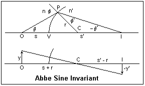 The upper diagram shows a ray from the object point O, to a spherical refracting surface at P, and then to an image point I. This is an actual, finite ray and not a paraxial approximation. We apply the Law of Sines to the triangles OPC and IPC. In OPC, r/sin θ = (s + r)/sin (π - φ) = (s + r)/sin φ, while in IPC r/-sin θ' = (s' - r)/sin φ'. Snell's Law is n sin φ = n' sin φ, which allows us to determine θ' in terms of θ for any meridional ray (ray that lies in this plane).
The lower diagram shows the ray from a point on the object at height y to the image point at height -y', which passes through the centre of curvature C, so that it is undeviated. The linear magnification m = y'/y = -(s' - r)/(s + r). We can use the results of the preceding paragraph to conclude that y/y' = r(sin φ'/sin θ')(sin θ/r sin φ). Using Snell's Law, we find that y/y' = n sin θ/n' sin θ', or ny sin θ = n'y' sin θ'. Since this holds at every refracting surface in the system, we have ny sin θ = constant, which is Abbe's invariant. Jenkins and White call it "Abbe's sine condition", which it is not; it holds for any system.
If the lateral magnification y'/y is to be the same for any ray, whatever θ, then n sin θ/n' sin θ' = constant, or sin θ'/sin θ = constant, since n/n' is a constant. This ratio must be independent of θ for constant lateral magnification, which is Abbe's sine condition. If it is satisfied, then the system is free of the aberration of coma, provided spherical aberration is also absent. It is often evaluated by plotting sin θ' as a function of the height h of an incident ray parallel to the axis. The plot should be a straight line. The distances h/sin θ' = f' can be compared with the paraxial focal distance H'F' as a measure of coma.
Aberrations
Since we are going to talk at length about it, it seems proper to review the spherical mirror. According to our conventions, a concave mirror has a negative radius, and a convex mirror at positive radius. The focal length in either case is f = -r/2, which assigns a positive focal length to the concave mirror, a satisfactory result, since a concave mirror converges light. Object and image distances, and focal lengths, are positive when measured to the left of the vertex. Then, as usual, 1/f = 1/s + 1/s', and m = -s'/s. When you look at your face in a shaving mirror, an enlarged virtual image is seen as if behind the mirror, while your face is less than the focal length in front of the mirror. An object at s = 2f is imaged with magnification m = -1 at s' = 2f: immediately below the object. It is instructive to draw ray diagrams for these cases. The primary and secondary focal points F, F' coincide for mirrors.
When you look into a convex mirror, you see a reduced virtual image of your face there. These mirrors are often used to present a wide field of view, and bear a legend: "objects seen in this mirror may be uglier than they appear"--sorry, "closer than they appear". This happens for any object distance, and the virtual image is between the vertex and the focal point just behind the mirror.
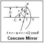 Exact ray tracing for spherical mirrors is quite easy. Consider a horizontal ray of height h incident on a mirror of radius r (here taken positive to avoid a lot of unimportant minus signs). The reflected ray crosses the axis at a distance r - r/2 cos θ = (r/2)(2 - sec θ) = r/2 - rθ2/4, approximately. θ is the angle between the radius to the point of reflection and the axis. The paraxial focal length is r/2, and the spherical aberration is rθ2/4. Note that it increases as the square of the angle θ--that is, quite rapidly.
A convex mirror can be analyzed similarly. The incident ray at height h is reflected to slope upwards at an angle of 2θ, where sin θ = h/r, and the isosceles triangle again gives us f = (r/2(2 - sec θ), or r/2 - rθ2/4. Just as in the case of the concave mirror, the focal point approaches the vertex as h increases. Since the focal point is to the right of the vertex, it is considered negative in the lens equations.
From the ray tracing, we find that h/sin θ' = h/sin θ cos θ = r/cos θ. Since this is not constant, but varies with h, the spherical mirror does not satisfy the Abbe sine condition, and so will suffer from coma.
It is very instructive actually to view the images formed by a concave mirror. I used a shaving mirror of 150 mm diameter and focal length about 250 mm, with a flashlight as a source. The flashlight was placed about 8 metres away from the mirror, and aimed at the mirror, so it formed a point source about at infinity. The images were caught on a piece of white paper. It was very clear that the mirror was not perfect from the nature of the images. When the mirror was adjusted so the light struck it normally (or nearly so, since the screen would obstruct the light), the paraxial focal point was easy to estimate, and moving the screen back and forth revealed the shape of the cone of light, bounded by the caustic surface, and clearly showing the spherical aberration.
 The off-axis images were more interesting. Comatic flare was observed, as we expected. Most interesting were the image lines, the astigmatic images. The sagittal line was normal to the plane of the rays and the axis, as expected, and was first seen as the screen approached the mirror. Then, as the screen was moved toward the mirror, there was a rather large region of light that resolved itself into a line perpendicular to the sagittal line. This was the tangential astigmatic image. With some care in observation, we would find that the sagittal line was in focus over a plane normal to the axis, while the tangential line focused over a spherical surface tangent to this plane. In fact, the distances along the chief ray to the focal points is (r/2)cos θ (T) and r/(2 cos θ) (S), as shown in the diagram. This is proved in Monk (see References).
The same thing can be done with a reading glass, say about 100 mm in diameter and with a focal length of 250 mm. These are usually double-convex lenses. Again, any sufficiently distant small light is a good source. I used the porch light of a house across the street. Examine the paraxial focal point, and again observe the spherical aberration, which will be less than for the mirror. When the lens is rotated, an excellent comatic flare will be seen that is very much like theory predicts. This will be mixed with evident astigmatic lines, the T line nearer the lens than the S line. The cone of rays near the paraxial focal point will show a spectrum, red on the outside and blue on the inside, as expected.
The f-number of a focusing instrument is the ratio of the focal length f to the diameter of the entrance pupil (the aperture that limits the incident rays) D. For example, if f = 1000 mm and D = 100 mm, the instrument is said to be f/10, since 1000/100 = 10.
Suppose we place a circular aperture of 100 mm diameter at the centre of curvature of a concave mirror of focal length 1000 mm (that is, of radius 2000 mm). The diameter of the mirror should be a good deal larger than the diameter of the aperture. For light entering at some angle, the aperture guarantees that it will strike the mirror normally, and so have no more aberrations than light entering along the axis. This forms a lensless Schmidt system that will provide a wide field of view with a good quality image. The focal surface is, of course, curved, and the recording medium must allow for this. The aperture f/10 is tpical for such systems.
Instead of a simple aperture, a Schmidt system places a glass corrector plate at the centre of curvature. The corrector plate must be specially figured to do its duty, which is to eliminate spherical aberration on reflection. This permits a smaller f-number and consequently a greater speed due to the increased illumination. Schmidt systems are very popular for astronomical survey work, and several modifications have been devised. They were invented by Bernhard Schmidt in the 1930's. The corrector plate does not introduce enough chromatic aberration to be troublesome. With the spherical aberration eliminated, the coma and astigmatism are also small.
Another way to reduce the spherical aberration of a concave mirror is to silver the back side of a negative meniscus. The combination is called a Mangin mirror. The glass protects the reflecting coating, which is specially advantageous in searchlights when an arc lamp is used. In a typical example, the first radius is -r, the second -1.5r. In the paraxial approximation, the concave meniscus has a focal length -6r, assuming n = 1.5, while the mirror has a focal length 3r/4. Since the meniscus is traversed twice by the light, the focal length of the combination will be 1/f = -1/6r + 4/3r - 1/6r = 1/r. That is, the focal point is at the centre of curvature of the first surface. The concave mirror and diverging meniscus have opposite spherical aberration, so the net spherical aberration is reduced.
The algebraic theory of aberrations is very complex, and it is not easy to arrive at easily comprehended results. Exact ray tracing can easily be done on a computer, and is an indispensble resource. However, it only gives mountains of data for a specific system, not general results. The possibility of optimization allows the fine-tuning of an established design, but does not suggest innovative solutions. The classical process is to add cubic and higher terms to the paraxial analysis. For example, sin θ = θ + θ3/3! yields the third-order results. We must also take the shape of spherical refracting surfaces into account, and no longer consider them planes.
Five third-order primary or Seidel aberrations are recognized, which seldom appear individually. They are called spherical aberration, coma, astigmatism, curvature of field and distortion. Which are of importance depends on the instrument. Telescopes, microscopes and similar make images close to the axis, and are most affected by spherical aberration and coma. Cameras and other wide-field instruments are more affected by astigmatism, curvature of field and distortion. Nevertheless, the elimination of spherical aberration is usually the most important aim. For given object and image distances this can be done exactly, by using aspherical surfaces. Except in a few cases, this is undesirable. Aspheric surfaces are expensive to create (recently, the possibility of good cast plastic lenses reduce the cost in mass production), and give notably poorer results if used outside their specific design conditions.
Spherical aberration in lenses can be minimized by choosing the proper lens shape, or "bending" the lens without changing its power. The shape factor q = (r2 + r1) / (r2 - r1) can distinguish lenses of different shape with the same power (n - 1)(1/r1 - 1/r2). q = 0 corresponds to a biconvex lens, r2 = -r1. q = 1 means r2 = ∞, or a planoconvex lens with the curved surface facing the incident parallel light. q = -1 is the same lens, but turned around. Smaller and larger values of q designate meniscus lenses. For parallel light in, minimum spherical aberration occurs for q about 0.75, very close to the planoconvex lens. As a general rule, minimum spherical aberration occurs when the bendings at each surface are equal.
Coddington defined a position factor p = (s' - s)/(s' + s) that varies from -1 to +1, and found that the minimum spherical aberration occurs for q = [-2(n2 - 1)/(n + 2)]p. For n = 1.5, this is q = -1.3p, and for n = 1.6 it is q = -0.87p. For p = -1 (object at infinity), something around q = 1 will be best. This is a plano-convex lens with the curved surface facing the parallel light, as already noted.
 To see vividly what the aberration of coma is, make a mask like the one shown in the figure. The dimensions are not critical. I used a central disc of 10 mm radius, and the zone of radii 35 and 40 mm. The mask can be cut out of ordinary paper, and tacked on the reading glass with "glue stick'. Throw the image of a distant lamp (for me the porch light across the street) on a piece of paper taped up so you don't have to hold it. Find the focal point and align the lamp for a symmetrical image. This should be a rather sharp image since the lens has been stopped down to about f/12.5 rather than the f/2.5 for the whole lens.
Now rotate the lens to one side or the other. A loop of dim light will be thrown out to one side or the other. This is a comatic circle, made by the light passing through the annular space in the mask. To prove this, occult a small part of the annular space with a finger, and a small interval of the comatic circle will disappear! Even more curiously, as you go around the annular mask once, you go around the comatic circle twice. It is not hard to discover what parts of the annulus correspond to what parts of the comatic circle. In the absence of the mask, each zone of the lens will make a comatic circle of a radius proportional to the distance from the vertex. This is how the comatic flare is built up. Coma occurs for relatively small departures from the axis, before astigmatism becomes a problem. If you rotate the lens further, you can probably see the onset of astigmatism, which is mixed with the coma.
The index of refraction of transparent media varies with the wavelength of the light, generally decreasing as the wavelength increases, approximately described by Cauchy's formula, n = A + B/λ2 + C/λ4. The middle of the visual spectrum is taken to be the Fraunhofer D line, due to Na, at 589.0 and 589.6 nm. Its limits are the red C line at 656.3 nm and the blue F line at 486.1 nm, both due to H. These wavelengths are selected because of the wide use of the Fraunhofer lines as standard wavelengths that are easily reproduced. The dispersion constant ν = (nD - 1)/(nC - nF) is a convenient measure of the index relative to the dispersion over the visible spectrum. Its reciprocal could be called the dispersive power.
The familiar soda-lime glass used for windows and eyeglass lenses was called crown glass from its original method of manufacture as circular sheets, where the residue around the rod when the glass was removed looked like a crown. The word was later used for many types of glass with similar constitutions, even the later boron. Its typical index of refraction for D light is 1.5, and its ν = 60. Flint glass, which contained lead or barium, was used for decorative cut glass, for which its high index of refraction, around n = 1.65, suited it. For these glasses, ν was significantly lower, as low as 35 or 40. This means that the dispersion increased more rapidly than the index. Glasses now contain lanthanum or titanium, and can be obtained with indices up to 2.0 and ν from 15 to 95. Water has nD = 1.33309 and ν = 55.6 at 20°C.
It will be convenient to write the lensmaker's equation as P = (n - 1)K, where P = 1/f is the power (in diopters if f is in metres), and K = 1/r1 - 1/r2. For a small variation dn in the index, dP = Kdn, or dP/P = dn/(n - 1). If dn is the variation across the visible spectrum, then dP/P = -df/f = 1/ν, or df = f/ν (ignoring the sign). For a lens of long focal length, as was used in refracting telescopes, this means that the focal length will be significantly different from red to blue. If f = 1000 mm, then df = 16.7 mm for the typical crown glass lens used in early telescopes. This longitudinal chromatic aberration was clearly extremely unsatisfactory. The differences in focal length also meant differences in magnification, so blue images were surrounded by a border of red. This is called transverse chromatic aberration. It is possible to make the focal points coincide without making the focal lengths equal, which will leave transverse chromatic aberration that may be annoying. This problem was the stimulus for Newton's invention of the reflecting telescope, which does not suffer from chromatic aberration.
 It is easy to achromatize a thin lens by combining a converging lens of crown glass with a diverging lens of flint glass. New glasses were devised (notably by Schott of Jena) that made this combination very effective. The ray diagram at the right may help to make the method clear. A horizontal ray from the left is refracted by the converging lens toward its secondary focal point F1'. A parallel ray through the centre of the lenses strikes the focal plane of the diverging lens that passes through its secondary focal point F2' and defines the virtual image for the diverging lens. A ray from this point through the point where the incident ray strikes the converging lens meets the axis at F', the focal point of the combination. Now, if the focal length of the converging lens decreases slightly, the parallel ray becomes a bit steeper, intersecting the final ray a little closer to the lens. If the focal length of the diverging lens changes by the proper amount, then the final ray is not changed and F' remains at the same position.
This can be seen analytically as follows. For the two thin lenses in contact, P = P1 + P2, so the condition for achromatism is dP = dP1 + dP2 = 0. Dividing by the product P1P2, we find 1/ν1P2 + 1/ν2P1 = 0, or P1/P2 = -ν1/ν2. This shows that the powers of the two lenses must be opposite in sign, and also if ν1 > ν2, P1 is greater than P2 so that the net power P1 + P2 will be positive. If we know ν1 and ν2, and the net power required P, we may determine the separate powers P1 and P2.
Suppose we want P = 10D, or f = 100 mm, and we choose glasses with ν = 60 and 40. Then, P1/P2 = 1.5 and P1 + P2 = 10, from which P1 = +30D (f = 33.3 mm) and P2 = -20D (f = -50.0 mm). There are four radii available. The Gauss lens, an excellent telescope objective, is a spaced doublet with a meniscus crown converging lens followed by a meniscus flint diverging lens so all four radii may be different. It is often convenient to make r3 = -r2 so the lenses fit together in contact. We can satisfy the conditions on the powers by fixing two more radii, which still leaves one radius free to be chosen. This makes it possible to choose the lens shape to minimize the spherical aberration, and this is usually done. The result is called an achromat, which not only is corrected for chromatic aberration, but for spherical aberration as well. As a bonus, coma is usually quite small as well. Lenses for critical duties should be achromats, even if the illumination is monochromatic. Since it may be difficult to find achromats off-the-shelf for arbitrary object and image distances, another trick is to use two achromats designed for an infinite distance on one side but the desired distances on the other sides.
A Cooke triplet (1893) consists of a flint diverging element between two crown converging elements. All the primary aberrations can be corrected with this design. The Zeiss Tessar (1902) is similar, but with a doublet third lens. The triplet can be made symmetrical by dividing the flint negative element into two separate lenses. An aperture is usually placed at the centre between the negative elements. Symmetrical systems minimize distortion, so they are often found as camera lenses. An example is the Dogmar-Avlar or Celor lens, consisting of four spaced elements. With camera lenses, a flat field is a primary consideration. In early inexpensive cameras, a stop in front of a simple concave positive meniscus lens gave a flat field for rather small apertures, f/11 at the most. This was called a landscape lens. Using a meniscus achromat gives a sharper image. These lenses were usually corrected for the D and G (434.1 nm) lines to better suit photographic emulsion sensitivities, instead of the usual C and F lines. The rapid rectilinear lens, a symmetrical lens formed by two cemented doublets with the flint elements outermost and a stop in the centre, increased the speed to f/8.
There is also a way to achieve achromatism with only one kind of glass, using two separated thin lenses. If c is the distance between the lenses, we know that P = P1 + P2 - cP1P2. If we differentiate this expression, set it equal to zero, and then solve for c, we find that c = (dP1 + dP2)/(P1dP2 + P2dP1). If we divide top and bottom by P1P2, and remember that dP/P is the same for both lenses, we find c = (1/2)(1/P1 + 1/P2), or c = (f1 + f2)/2. That is, if two converging thin lenses are separated by half the sum of their focal lengths, then the combination has the same focal length for a range of wavelengths around the one for which the focal lengths were given.
An eyepiece or ocular is a component that renders the divergent rays from a real image produced by a telescope or microscope objective parallel, so that they can be focused by the eye. That is, it is a magnifier. It may be a single lens, divergent and placed in front of the image in the Galilean telescope, or convergent and placed behind it in the Keplerian telescope. Two or more lenses or lens combinations are used in the more elaborate eyepieces. The two lenses are called the field lens and the eye lens; the eye lens is the one closer to the eye. In the Huygens eyepiece, the lenses are plano-convex with the convex surfaces forward, and with fl/fe = 1.5 to 3.0. In the Ramsden eyepiece, the convex sides of the plano-convex lenses of equal focal length face each other. The lenses are usually a little closer together to move the focal plane forward away from the field lens, at the expense of less perfect achromatization. A reticle or crosshairs can be placed at the focal plane if this is done for direct comparison with the real image. Although these eyepieces were adequate, they were by no means perfect and more elaborate designs were developed. These still usually consist of two lenses, of which one or both are achromatic doublets or triplets. The classic Kellner and Abbe orthoscopic eyepieces are still good choices for general use. The eye relief is the distance between the last lens surface and the exit pupil, where the pupil of the eye should be placed. It should be at least 6 mm, and more if possible.
The astigmatism we have discussed so far has been due to the different curvatures of the refracting or reflecting surface in the sagittal and tangential planes as a result of incidence at large angles from the axis. The refracting or reflecting surface may not have the same curvature in all sections even on the axis; in this case, the image will be astigmatic even for paraxial rays. This occurs, notably, for the cornea of the eye. In this case, there is no stigmatic image for any focus, which causes blurred vision. Fortunately, the astigmatism is usually very small in this case, and can be easily corrected. If we consider the curvature of the refracting surface for different azimuthal angles, one plane will give a minimum radius of curvature, while the perpendicular plane will show a maximum radius of curvature. This is characteristic of a quadric surface. The result will be two focal lines for rays in these planes. Neither can be called sagittal or tangential in this case. The optometrist determines the azimuth of maximum radius of curvature, and corrects the refraction with a cylindrical lens so that it has the same power as the perpendicular section. Now the image will be stigmatic and needs only to be thrown on the retina by the use of spherical lenses.
When the usual astigmatism is eliminated, the S and T focalsurfaces coincide on a paraboloid called the Petzval surface. The curvature of this surface is often a disadvantage, and is considered one of the five primary aberrations. Moreover, the magnification (dependent on the focal length) may also depend on distance from the axis. If the magnification increases with distance from the axis, the corners are stretched relative to the rest, and we have pincushion distortion. If it decreases, then the result is barrel distortion. This is the fifth and final of the primary aberrations.
 An interesting construction for the refracted ray at a spherical interface is illustrated at the right. It was published by Thomas Young in 1807, but Jenkins and White attribute it to Huygens, and it was also used by Weierstrass. The surface of radius r separates media of indices n and n'; we assume n' > n here. Draw circles of radii rn'/n and rn/n' about the centre C of the surface. The incident ray meets the surface at A. Extend this ray until it meets the larger circle at B, and then draw the radius BC. This ray intersects the smaller circle at D. The refracted ray is AD, extended.
The key to the proof of this construction is that triangles ABC and DAC are similar, since corresponding sides are proportional. That is, CA/CN = CM/CA = n'/n. Therefore, the angles CAD = φ' and ADC = φ are the angles of refraction and incidence, respectively. The same angles appear in triangle ABC, of course. Since the sides of the triangle are r and rn/n' as shown, the Law of Sines immediately gives n sin φ = n' sin φ', which is Snell's Law. If this is not completely clear, make a careful drawing, copy it, and cut out the small triangle ADC. Then fit this triangle over the large triangle ABC and note the corresponding angles.
Imagine the incident ray rotated until B and D fall on the axis. Then, any ray directed towards B will be refracted to pass through D. This is a remarkable result: The image D of the virtual object B is perfectly stigmatic. Points like B and D are called conjugate aplanatic points. They are made use of in an oil-immersion microscope objective where they form the first stage of magnification.
 Young's construction is really rather convenient. It is applied to a biconvex thick lens in the diagram at the left. Notice that for the right-hand interface the roles of the construction circles are interchanged. The circles at the right refer to the first surface, those on the left to the second surface. The intersection of the incident horizontal ray at height h with the final ray locates the secondary principal point H'. Try this on a lens with n = 1, n' = 1.5, r1 = -r2 = 30 mm, d = 20 mm. The paraxial focal length is 27 mm, while for h = 15 mm, the construction gives f = 24 mm, and H' 5 mm in front of the second vertex. It is easy to see spherical aberration and curvature of the principal plane.
The aplanatic points of a reflecting ellipsoid of revolution are its foci. If one focus recedes to infinity, then we have a paraboloid. For a plane mirror, every point is an aplanatic pair with its virtual image. For a concave spherical mirror, the centre of curvature is aplanatic with itself. For any two points in different media, there is a refracting Cartesian oval that makes them an aplanatic pair. In every case, the optical path length is the same on every ray joining conjugate aplanatic points.
References
There are newer editions of the following two texts, but these are the editions I like to use.
E. Hecht and A. Zajac, Optics (Reading, MA: Addison-Wesley, 1974). For Smith matrices, see pp. 171-175.
F. A. Jenkins and H. E. white, Fundamentals of Optics, 2nd ed. (New York: McGraw-Hill, 1950). Chapters 3-6 and 9.
B. E. A. Saleh and M. C. Teich, Fundamentals of Photonics (New York: John Wiley & Sons, 1991). Sec. 1.4, pp 26-37. The ray vector used here is [h θ].
G. S. Monk, Light, Principles and Experiments, 2nd ed. (New York: Dover, 1963). Appendix III, pp 424-426, for astigmatic focal surfaces.
The Wikipedia article on aberrations is not very good; it seems to have been copied from an old encyclopedia. The article on eyepieces is quite good, with excellent links.
Return to Optics Index
Composed by J. B. Calvert
Created 4 September 2007
Last revised 6 September 2007