Wind

An exploration of the wind

Contents

1. Introduction
2. Measuring Winds
3. The Geostrophic Wind
4. The Gradient Wind
5. Effect of the Surface
6. The Thermal Wind
7. The Isallobaric Wind
8. Local Winds
9. Winds of the General Circulation
10. Tornadoes
11. Tropical Storms and Hurricanes
12. The Beaufort Wind Scale
13. The Force of the Wind
14. References

I wanted to know a little more about the wind, to consider its effect on sound propagation, so I looked up the fundamentals, and here is my interpretation of them. There appear to be three branches of the subject: (1) dynamics of the wind well away from the surface; (2) the effect of the surface, and the formation of what is actually a boundary layer governed by viscosity and turbulence; and (3) special winds. Wind is of great importance in meteorology, of course. This article has expanded with time, and now contains considerable information on tropical storms and tornadoes.

The principal wind characteristics are speed and direction. The direction of a wind is the direction from which it blows. A north wind comes out of the north and blows southward, while a west wind comes out of the west and blows eastward. Wind direction is best described by its azimuth, measured clockwise from north from 0° to 360°. A wind of azimuth 200° blows from the SSW; a wind of azimuth 45° blows directly from the NE.

An approximate means of expressing wind direction that is usually quite accurate enough is to use points of the compass in the wind rose, a 16-point example of which is shown at the right. SSW is south-southwest, azimuth 202-1/2°. More crudely, only 8 points could be used: N, NE, E, SE, S, SW, W, NW and back to N. Four points is a bit too crude. Wind direction is measured with a rotating vane; the direction can be telemetered using a rotary encoder, which is now the cheapest and easiest way. Repeating servomotors can also be used, but they cost more.

The wind rose antedated the compass. Around the Mediterranean Sea, certain seasonal, identifiable winds that blew in fixed directions could be recognized, and by means of these winds the orientation of the wind rose could be determined when there was no other clue. The cardinal winds were named Boreas (N), Eurus (E), Notus (S) and Favonius (W) in Latin. Winds were then interpolated between each of these to give 8 winds, and the idea was extended further with less success. The sun by day and the stars by night gave other indications, so the wind rose could usually be oriented to find the direction of sailing. When the magnetic needle arrived in the 13th century, it was used as just another way to orient the wind rose, and one that was often not trusted. The mariner's compass originated in the marriage of the wind rose floating in a bowl with the Chinese necromantic needle attached to it.

Wind speed is measured by an anemometer, of which there are many kinds. Most common was probably the 3-cup freely rotating anemometer that is calibrated in a wind tunnel. The force on a spring-loaded vane, or the pressure in a Pitot tube can also be used. Pressure sensors allow the design of a variety of anemometers whose data is easily telemetered. Whatever the design, an anemometer should be equally sensitive to winds from any direction. This is done by making the design naturally isotropic, like the 3-cup anemometer, or by turning the device into the wind with a wind vane. The standard height of the anemometer is 10 m. Wind speeds increase rapidly with altitude, and most anemometers are in the surface boundary layer. A more detailed discussion of the vertical wind profile will be found in Turbulence, as well as below in the section on surface effects.

Free balloons can be used for measuring upper winds by tracking them as they ascend. The rate of ascent is assumed known, and the position of the balloon is calculated from its altitude as measured by a theodolite. There are more modern ways of doing this that do not require such a skilled observer, and can be carried out by the idiots currently available. Unless the altitude of the balloon is determined by some independent source (radar, GPS), and not by timing on the basis of the free lift, the results cannot be expected to be accurate.

Wind speed is officially reported in knots, nautical miles per hour, apparently because of the connection with air navigation, even though traditional graphical navigational procedures that are facilitated by this unit are probably no longer used. A nautical mile corresponds to 1' of arc on a spherical earth, or 6080.20 ft. The equalities 1 m/s = 1.942 kt = 2.237 mph = 3.600 kmph will be found useful. The Beaufort scale, an excellent way to determine and express rough estimates of wind velocity that are often good enough for many purposes, is given in a later section.

Winds are also not steady, either in velocity or direction, and the description of these variations, sometimes quantitatively, may be desired. The mean wind velocity and its standard deviation are useful statistics with considerable meaning. The range of velocities is another statistic, or the interquartile range of velocities. Maximum velocities exceeded only a certain small percentage of the time may be useful, or the root-mean-square velocity, if the energy of the wind is of interest. Such statistics are obviously of interest in designing a wind farm, or other similar installation. The frequency response of the anemometer must also be taken into account; some give average values, while others are more responsive to fluctuations.

A wind is said to veer when its direction changes clockwise, and to back when the change is anticlockwise, in the northern hemisphere. In the southern hemisphere, the behavior is opposite. Veering can be described as "sunwise" motion in either hemisphere. If a low passes west to east north of you, the wind will be southwesterly, then westerly, then northwesterly, so the wind will veer. When a low passes south of you, again west to east, the wind will be southeasterly, easterly, and then northeasterly, again veering. If a low passes directly overhead, the southerly winds will fall, then northerly winds will replace them. Since the weather generally moves from west to east in temperate latitudes, and consists mainly of lows, a veering wind is the usual thing. It might be interesting to correlate the winds with the TV weather forecast.

The atmosphere is, of course, a compressible fluid, of low density and low viscosity, that obeys the ideal gas law to a good approximation. Let's describe its state in the Eulerian fashion by giving the pressure p, temperature T and vector velocity v as a function of position and time. Then, p = p(t,x,y,z) and similarly for the other quantities. These quantities must satisfy certain equations. First, the conservation of mass demands that ∂ρ/∂t + div(ρv) = 0, which is the differential way of saying that the mass within any closed boundary changes only because of the flow of mass across the boundary. ρ is the density of the air in g/cc and v the velocity in cm/s. This is called the equation of continuity, which must be satisfied by any wind flow. The pressure, temperature and density of the air are connected by the equation of state, p = ρRT, where p is in dyne/cm², T is in K, and R is the gas constant for air, R*/M, where R* is the universal gas constant, 8.3144 x 10⁷ erg/mol-K and M = 28.97 g, so that R = 2.870 x 10⁶ erg/g-K.

The third set of equations that must be satisfied are the equations of motion, dv/dt = -grad(p)/ρ - 2ω x v, where the two forces that always act on the air are included. The first is the pressure gradient force, which acts in the direction of the maximum change in pressure, while the second is the Coriolis force, a force which allows us to consider the earth as a nonrotating coordinate system, although it rotates with an angular velocity 7.292 x 10^-5 radians per second about an axis through the geographical poles. The direction is given by the vector relation, which is in the horizontal plane, and the magnitude is 2ω sin &phi, where φ is the latitude, tending to turn the velocity to the right in the northern hemisphere, or to the left in the southern hemisphere. This force is a maximum at the poles, and is zero at the equator. There is also the gravitational force -ρg, but this is usually balanced by buoyancy; when it is not, it must also be included. If the path of the air is curved, it is also subject to the centrifugal force v²/r. The equation of motion is written for one gram of air, and all the forces given are forces per gram.

The derivative dv/dt is not the usual time derivative of a function, but is the acceleration following a particle of fluid in its motion. In terms of the Eulerian functions, d/dt = ∂/∂t + v·grad is the substantial derivative that takes into account change due to the motion of the particle. Any hydrodynamics text will explain this in detail. It is the second term that makes the equations of motion nonlinear, and introduces so much difficulty into hydrodynamics. In our application, the velocities or time variations are small enough that we can often neglect the second term, thereby linearizing our equations.

The atmosphere is free and unrestrained by boundaries, only by the attraction that holds it to the earth and causes the density to decrease rapidly with height. This means that a very small horizontal force, acting for relatively short times, could give rise to very high velocities, which are not observed. We must conclude that most of the movement of the atmosphere, the winds, is mere coasting under no force. The pressure varies by only a small amount in any horizontal plane, and the Coriolis force is so small that it is scarcely sensible, but these forces act so widely that they control the winds. A difference of pressure is the only agency that can cause a wind; the Coriolis force acts perpendicular to the velocity (like the magnetic force on a moving electron) and cannot affect the velocity. Nevertheless, when we analyze winds we seldom if ever explicitly consider the forces that gave them motion; these forces perhaps acted for short times and far away, but their winds coast on continually. That some forces must act is shown by the proverbial fickleness of the wind, that is constantly varying in strength and direction.

We must assume, then, that the pressure gradient forces that we know must act because of the lateral variation in atmospheric pressure are exactly balanced by the Coriolis force, so that we have a time-independent flow. In this case, -grad(p)/ρ = 2ω sin φv, which we can write (1/ρ)∂p/∂n = lv, where l = 2ω sin φ, and n represents distance normal to the isobars, while v is the velocity parallel to the isobars. The constant l depends only on the latitude. This equation gives the wind velocity v in terms of the pressure gradient and the density. The balance of forces is illustrated at the right. This wind is called the geostrophic, or "earth-turning" wind, and is of fundamental importance. We know the velocity and direction of the wind if we know only the pressure distribution, which is remarkable. The forces causing the wind do not play a part in our analysis.

In general, when a wind is blowing towards you, the low pressure is on the right hand. Buys Ballot's Law, that the low pressure is to your left when your back is to the wind, is simply the inverse of this. Note that the diagram above is consistent with these statements. These qualitative predictions of the equation are well borne out in practice, and wind speeds are usually predicted from the density of the isobars.

Pressure is usually measured in millibars, 1 mb = 10³ dyne/cm². Distance is conveniently measured in the length of a degree of latitude, which is 111 km or 69 mi. Then, a pressure gradient of 1 mb per degree of latitude is 8.993 x 10^-5 dyne/cm²/cm. The isobars on a weather map are usually drawn with a 4 mb contour interval, so to get the pressure gradient we multiply the above figure by 4 divided by the distance between the isobars in degrees of latitude. Of course, we can easily adjust this if we use km or miles instead. The constant l = (2)(7.292 x 10^-5)(sin 40°) = 9.374 x 10^-5 s^-1. The density of air in Denver under normal conditions is close to 10^-3 g/cc, so I shall use this round figure. The density at STP is 1.293 x 10^-3 g/cc. Therefore, the geostrophic wind at Denver under normal surface conditions is 959(∂p/∂n) cm/s, where the pressure gradient is in mb per ° of latitude. Since 1 m/s = 1.942 kt, this is also 18.6(∂p/∂n) kt.

In explaining the geostrophic wind, we assumed that the isobars were straight lines. This is seldom the case in practice, so we must allow for curvature of the isobars, which introduces centrifugal forces, and thus a cyclostrophic component to the winds.

A cyclone or low is an area of closed isobars surrounding an area of lower pressure. The wind blows along the isobars in the direction in which the pressure gradient balances the Coriolis force. The pressure gradient force is inward, so the wind must blow anticlockwise around the cyclone. An anticyclone or high is the opposite case, and now the wind must blow clockwise so the forces can balance. Let's consider circular isobars making idealized cyclones and anticyclones. The balance of pressure gradient, Coriolis and centrifugal forces for a cyclone gives (1/ρ)∂p/∂r = lv + v²/r. This is a quadratic equation for v, of which the meaningful solution is v = -lr/2 + √[l²r²/4 + (r/ρ)(∂p/∂r)], where r is the radius, and where we use the radial gradient of pressure.

For an anticyclone, the force balance is (1/ρ)(∂p/∂r) + v²/r = lv. The solution for v is v = lr/2 - √[l²r²/4 - (r/ρ)(∂p/∂r)]. If the pressure gradient is too large for a given value of r, the quantity under the radical may become negative, which cannot be allowed. In fact, large pressure gradients are never seen at the centres of anticyclones. For a given radius and pressure gradient, wind velocities are higher for anticyclones than for cyclones.

When centrifugal forces due to curved isobars are taken into account, the winds are called gradient winds, a term that includes the geostrophic winds as well.

The wind speed must decrease from its free velocity V to zero at the ground. The wind gradient implies a retarding, or frictional, force on the wind that has an important effect on wind strength and direction. A look at a surface analysis chart will show that winds apparently do not know that they should follow isobars. Sometimes they do, more or less, but more often than not seem to move independently, especially if they are weak, say below 20 kt. On the other hand, winds 100 m or more above the surface will be seen to follow isobars very closely, and the wind velocity will agree very well with the equation we have found for the geostrophic wind. This is very well seen at the 250 mb level with the jet stream winds.

The velocity profile near the surface is determined mostly by turbulence, which is very effective in transporting momentum. For a discussion of turbulence, see Atmospheric Turbulence. We'll just use the results here. When a wind is blowing, a laminar boundary layer is formed near the surface which is dominated by the molecular viscosity of the air. There is a relatively large velocity gradient in this layer, but it is not very thick. If irregularities on the surface are completely immersed in this laminar boundary layer, their size does not matter, and the surface is aerodynamically smooth. Larger bodies may project through the layer, and retard the wind by form drag like any large body in an airstream. If these bodies dominate, then a turbulent boundary layer is formed, of a thickness we shall denote by ε, and the surface is classed as aerodynamically rough. Meteorologically, the earth's surface is generally rough, except that a calm sea surface may be smooth.

The velocity profiles under different condtions are sketched at the left. The wind velocity above the effect of the surface is V, and z = ε is the height at which v = 0. The velocity profile is often expressed empirically as u = u'(z/z')^p, where u' and z' are constants, and u is the velocity at height z. In the case of laminar flow, which occurs for a very stable atmosphere (isothermal or inversion), p = 1, and the wind velocity increases linearly with height. For very unstable air, strong turbulence makes p = 0, so that the velocity is independent of height, except for a thin transition layer that extends to a height z₁. Over a grassy plain, ε is 1-2 cm and z₁ is no more than 30 cm. These extreme cases are not usually encountered, but represent good limits.

In the intermediate case, the velocity profile is found to be logarithmic. A theoretical expression for the velocity is u = (v*/k)ln(z/ε). Here, v* is the friction velocity √(τ/ρ), where τ is the shear stress at the v = 0 plane and ρ is the density. k is the von Kármán constant, which has the value of 0.4, approximately. For grassy plains, we may assume v* = 40 cm/s and ε = 1 cm, so that u = 100 ln(100z), where z is now in metres. In knots, this is about u = 2 ln(100z) kt. The constants used here are only illustrative, and may vary widely. The diagram above shows the logarithmic velocity profile, which is followed up to the free velocity V. The transition is, of course, not abrupt in practice. For a 10 kt wind, z is only 1.5 m, for a 20 kt wind, z is 220 m, and for a 30 kt wind z is 3270 m, well out of the range of applicability of the formula. Note that the choice of ε is not critical, since it appears in the logarithm, and is usually small compared to the altitudes of interest anyway.

This velocity profile has consequences for the measurement of wind speed. For either of the extreme cases, the anemometer will give the true value of V if it is at a reasonable height, above z = z₂ where the linear profile ends in the laminar case. For the intermediate cases, the wind velocity at any level will not depend on the free wind velocity if the anemometer is below z₃ for that wind velocity. z = 1 m corresponds to 9.2 kt, 2m to 10.6 kt, 5 m to 12.4 kt, 10 m to 13.8 kt, and 30 m to 16.0 kt. The wind speed remains at these values for any larger value of V. An anemometer at 10 m, about 30 feet, will read no higher than 14 kt, no matter what V may be, as long as the logarithmic law holds. Of course, in higher winds we may approach the p = 0 case of high turbulence. The correlation of the wind speed observed with an anemometer to the free wind speed is a difficult subject.

Now we wish to consider the effect of ground friction on the geostrophic wind. This has been analyzed on the basis of turbulent transfer of momentum (from the air to the surface) with a constant eddy kinematic viscosity K. The result is the Ekman spiral that shows the direction and magnitude of the wind as a function of height. The wind direction turns to cross the isobars from high to low pressure, up to a maximum of 45° as the surface is approached and the velocity becomes small. This theory has been observed to be inaccurate, and has been redone assuming that K is a function of z (which it is). However, a simple derivation that shows the most important qualitative effects is possible, which we shall now present.

If we make the simple assumption that the equivalent frictional force on the air is proportional to the wind velocity, say f = -kV per gram, then we can include this force with the pressure gradient and the Coriolis force. The three forces then sum to zero, as shown in the figure at the right. Note that V is not a force. In the right triangle, we have (kV)² + (lV)² = (1/ρ)(∂p/∂x) = lV', where V' is the geostrophic wind without friction. Therefore, V = [lV'/(k² + l²)]^1/2 and tan θ = lV/kV = l/k. In this case, a frictional force causes the wind to back through an angle θ, as well as to decrease in velocity. The difficulty with verifying this equation is the determination of the constant k, but it does show the general behavior. Since the wind now blows from high to low pressure, work is done on the air by pressure forces that is dissipated in friction with the surface.

It is clear that the wind velocity is low at the surface, and increases with height. Therefore, the "surface wind" is not well-determined and depends on the details of measurement. We have discussed the wind profile above, and its effect on anemometry. The anemometer and wind vane should be placed in plane, open surroundings at a standard height. I cannot find specifications in the references available to me, but no doubt such standards exist, especially for reporting surface winds at airports. If I had to make a recommendation, I would say that the wind instruments should be placed at an elevation of perhaps 10 m, on a slender pole, in an open area a distance of 100 m from any obstruction or building. This would at least give a "surface wind" at a reasonable height, as undisturbed by turbulence as possible. The mounting of wind instruments on roofs of buildings would be adequate if they were a sufficient distance above the roof, and if no taller buildings were nearby. However, this would also tend to measure the velocity at a higher level, so the wind velocity would be systematically larger. Perhaps by two measurements at different heights, the rate of change of velocity and direction with height could be estimated. Whatever is done, surface winds at different stations are probably not comparable for theoretical purposes unless great care is taken. Note that not only buildings, but vegetation and surrounding topography can affect the direction and velocity of wind, as well as create eddies and turbulence.

Although we have spoken mainly of the contact of the air and the solid surface, similar considerations apply to the ocean surface, and as well to layers of distinctly different velocity. The ocean surface is smoother than the land surface, which will mean lower friction. Also, the air above the ocean is much more stable, and turbulence will not be as effective. Therefore, frictional effects should be much less at sea, which can be seen in the wind reports from ships. Surfaces of wind shear will also give an effect similar to friction, but the momentum transfer may accelerate air as well as retard it. The top of the stable layer under a temperature inversion is one example of this. Beneath the inversion, the air is stable and the wind may be calm, while a gale is blowing above.

It has been observed in some places that the January wind is relatively constant through the 24 hours of the day, while the July wind is perhaps half as large during the night, but increases to a noon maximum near the January level. In either case, there is no corresponding diurnal barometric gradient variation, so this is a surface effect. If W is the surface wind, and G the geostrophic wind, the ratio W/G increases with temperature. W/G is less than unity, and varies so widely that no rule can be given. Values of .5 to .6 are frequent. Surface winds also deviate in direction from the geostrophic wind. At above 2 km altitude, the wind appears to be undisturbed by the surface, and turbulence is slight. Empirical formulas have been given for the variation of velocity with height, such as v = kh^α with α = 1/5 or 1/4. The variation is greater for stronger winds. The theoretical analysis is based on the transport of momentum from the geostrophic wind at altitude to the surface by eddies or turbulence. The diurnal variation is a result of the creation of turbulence by convection, and a consequent rise in the eddy conductivity. The equation for the propagation of momentum is ρ(du/dt) = d(κρ(du/dz))/dz (derivatives are partials), where κ is the eddy conductivity, on the order of 5 to 20 x 10⁴ cm²/s. The value is roughly wd/4, where w is the mean vertical turbulent velocity and d is the diameter of an eddy.

A "thermal wind" sounds as if it should be a wind caused by heat, but it is not. In addition to the variations of pressure over a level surface, there may also be variations of temperature. Isotherms can be drawn like isobars, and the two sets of curves can have any relation to each other. Now, it happens that the pressure aloft over different temperatures changes by different amounts, so that the upper isobars are rotated relative to the lower isobars, and this rotation changes the direction of the geostrophic wind. The difference between the geostrophic wind at altitude and the geostrophic wind at reference level is called the thermal wind component. It is not a whole wind in itself, just an amount that must be added to the geostrophic wind to get the wind at a higher level. This was once more important than it is now, when we can determine the winds at any altitude directly, and do not have to infer them.

The pressure, height and temperature are related by (1/ρ)(∂p/∂z) = -g/RT. We are interested in the change in the pressure gradients ∂p/∂x and ∂p/∂y with height, so if we take the derivative of the above expression with respect to x and y, and then invert the order of differentiation and use the ideal gas law, we will find (∂/∂z)[(1/ρ)∂p/∂x) = (g/RT²)(∂T/∂x) and (∂/∂z)[(1/ρ)∂p/∂y) = (g/RT²)(∂T/∂y). These equations relate the vertical changes in pressure gradients to the temperature gradients in horizontal planes. The y component v of the geostrophic velocity satisfies v = (1/lρ)∂p/∂x = (RT/lp)∂p/∂x. Dividing by T and taking the derivative with respect to z, we get ∂(v/T)/∂z = (g/lT²)∂T/∂x. A similar equation for the x component u is obtained, but with a change of sign and the y derivative of T.

If these equations are integrated from z to z', we can find the differences in the geostrophic velocities as integrals: v'/T' - v/T = (g/l)∫(z,z')(1/T²)∂T/∂x dz, and u'/T' - u/T = (-g/l)∫(z,z')(1/T²)∂T/∂y dz. With enough information, the integrals could easily be done numerically. However, approximate results may be good enough. We suppose the ratio T'/T can be replaced by unity, and that T can be replaced by its average value. If, furthermore, the temperature derivatives are approximately constant, then we find that: v' = v + (g/lT)(∂T/∂x)(z' - z) and u' = u - (g/lT)(∂T/∂y)(z' - z). In each case, the second term is called the thermal wind from level z to level z'. We see that it is parallel to an isotherm, since ∂T/∂n is normal to an isotherm, and is proportional to the horizontal temperature gradient.

If the wind blows from lower to higher temperatures perpendicular to the isotherms, then the thermal wind is perpendicular to the geostrophic wind, and the thermal wind turns the wind clockwise, or it backs. If the wind blows parallel to the isotherms (and the isobars), with low T corresponding to low p, then the isobars come closer together above, and the wind increases, but does not change direction. If low T accompanies high p, then the wind decreases at the higher level.

Thus far, all has been constant in time, and the winds are steady. Now we consider the case in which the pressure changes with time, and new winds are created. We are familiar with isobars, the lines p = constant, on the weather map. These curves are drawn from the station pressures also shown on the map. The station reports contain another item of pressure information, the "tendency" or change of pressure in 3 hours. The entry 14/ means that the pressure has risen by 1.4 mb in the last 3 hours at the station. We now have a representative value of ∂p/∂t at each station. These values can be contoured just like the pressure itself, and the lines ∂p/∂t = constant are called isallobars, lines of constant barometric tendency. Rates of change of pressure contour just like pressure itself, with highs and lows.

If you want isallobars, you usually have to draw them yourself. To do this, put a sheet of tracing paper over the weather map, and at each station put a dot to locate the station, and beside it the tendency at that station, being sure to assign the proper sign, + or -. When you remove the tracing paper, the tendencies will be much easier to interpret than on the cluttered map. If you have enough data, isallobars can then be drawn. We'll show in a minute how to use the resulting map.

We now go back to the equations of motion: du/dt = lv - (1/ρ)∂p/∂x and dv/dt = -lu - (1/ρ)∂p/∂y. The pressure gradient terms can be expressed in terms of the geostrophic velocities v' and u', so we have du/dt = l(v - v') = lv" and dv/dt = -l(u - u') = -lu". The double-primed quantities v" and u", which must be added to the geostrophic winds v' and u' to get the total winds v and u, are called the isallobaric winds. They are proportional to the acceleration of the air, so are the direct result of forces.

To make the equations soluble, we neglect everything after the first term in the acceleration du/dt = ∂u'/∂t + ∂u"/∂t + (terms like u∂u/∂x, etc). People who have considered this in more detail say this approximation is valid in most ordinary cases, so let's rely on their advice. Then ∂u'/∂t = -(1/lρ)∂²p/∂y∂t = lv", and in the same way, ∂v'/∂t = - lu". Solving for v" and u", we have the expressions v" = -(1/l²ρ)∂²p/∂y∂t, and u" = -(1/l²ρ)∂²p/∂x∂t. In vector notation, v" = -(1/l²ρ) grad(∂p/∂t).

The result is then quite simple: the isallobaric wind blows normal to the isallobars from high tendency to low tendency, and the velocity is proportional to the gradient. That is, there is divergence from an isallobaric high and convergence to an isallobaric low. Continuity tells us that in the first case, ther must be a downward flow, and in the other an upward flow. All this depends on rates of change of pressure, not on the pressures themselves.

An example is shown at the right. The isallobar contour interval is usually 1 mb/3hr. The wind is normal to the isallobars, and blows "downhill." Two isallobars are shown, with a distance between them of 100 km. From this we can estimate ∂²/∂n∂t and express it in cgs units. The derivative is just 1 mb/3hr/100km x (10³/3/3600/10⁷) = 9.26 x 10^-4 dyne/cm²-s. In the other factor, 1/l²ρ, we use l = 9.374 x 10^-5 (for 40° latitude) and ρ = 10^-3 g/cc (Denver), to get 1.138 x 10¹¹ s²cm³/g. The velocity of the allobaric wind is the product of these two factors, V = 1054 cm/s = 20.5 kt.

Before pocket calculators, this formula was arranged so that the usual graphical aids for calculating the geostrophic wind could be used, but this complicates things more than it facilitates them. For repetitive calculations, the above procedure can be expressed in terms of available quantities (such as the isallobar spacing in km) for convenience. However, the present method offers the advantage of checking the units, which must be carefully done.

The direction of winds that do not seem to follow the isobars can often be explained by the isallobaric wind, though numerical comparisons are difficult because of the sparsity of isallobaric data. The gradient wind must be added to the isallobaric wind to get the total wind, of course. An isallobaric low attracts winds, and is a region of convergence. The resulting rising air often results in instability, clouds and precipitation. A rapidly falling barometer is an indication of being in an isallobaric low. Conversely, a rapidly rising barometer is an indication of clear skies and good weather, as a result of the diverging circulation.

Local winds, as the name implies, occur in limited areas and are generally surface winds. They are caused by pressure differences, usually arising from temperature differences, and the winds blow across the isobars, often accelerating rapidly in a short distance. The Coriolis force does not usually have an important effect on local winds, since it has little time in which to act. Often the winds are given local names, which adds interest to their study. Some local winds are guided and affected by slopes, valleys and plateaus, others by the meeting of land and sea.

One surface wind met in many situations is the katabatic wind, which I have observed in impressive intensity in Boulder, Colorado, and which often occurs along the mountain front. It is, in fact, called a "Boulder wind." A similar wind on the Southern California coast is called the "Santa Ana." When the air in a valley cools by radiation at night, it becomes heavier than the air around it, and slides away, being replaced by warmer and lighter air from above. The body of air can accelerate to surprising velocities, of up to 100 mph. There are also anabatic winds, that blow up a heated slope. Anabatic winds may occur at the same mountain front in the morning, when the slopes are heated by the sun. This rising air triggers instability over the foothills in the morning, which is then blown eastward by the prevailing west winds as cumulonimbus develops, and then sails as far as Kansas and Nebraska through the evening with rain and hail.

The bora of the Dalmatian coast is another katabatic wind. The high plateaus are cold in winter, while the Adriatic is warm. The lapse rate over the water is often superadiabatic, so the descending air spilling off the edge of the plateau is still cooler than its surroundings when it reaches the coast, and the instability causes storms. Similar gusty, cold winds in northern latitudes are called the williwaw (not to be confused with the Australian willy-willy, which is a hurricane). The harmattan of the West African coast is also a dry land wind blowing from December to February.

A Föhn wind, the Chinook (Inuit for snow-eater), is a very common winter feature in Denver, Colorado, where it usually makes February a dry, sunny and warm month. The prevailing westerlies lose moisture in climbing the mountains, then warm up and dry out at the dry adiabatic rate on descent from the foothills at 9000 ft to the plains at 5000 ft.: just this descent would turn a freezing 32 °F into a pleasant daytime 54 °F, and the warming is usually greater than this, since the winds must climb to over 12,000 feet on their way. Lenticular clouds form in the lee of the mountains, often showing colourful opal-like hues in the afternoon sun. Conditions at Calgary, Alberta are quite similar, and Calgary also has an unusually warm and dry winter climate for its latitude, just as Denver does.

Cool air can flow down the slopes of a branched valley system like the water in the stream that made the valley. The flow can even reverse during the day, and the warm air flows upstream. This is seen, for example, in the valley of the Columbia River at Trail, B.C. Air flows down the valley from about 1900 to 1000, and up the valley from 1000 to 1900, with maximum velocities of 5-7 mph. The air in a confined mountain valley can radiate into clear skies and cool significantly, creating an inversion over the valley that allows warmer winds to pass over, while the floor of the valleys shivers. Cool air also drains in from the surrounding heights to fill the basin. This happens in the San Luis Valley of southern Colorado, which often is remarkably cold in winter.

Other local surface winds are associated with large convective storms. Precipitation may cool a volume of air through which it passes, which then acts katabatically, producing a sudden outward and downward rush, often seen in mammatus formations. Convection itself causes a wind inwards toward the centre of the storm. Roll clouds, or arches, may form around the periphery of the storm. There may be rotation in a horizontal plane as well, and lowering of pressure can produce a mesocyclone, a miniature rotating low. With sufficient rotation, whirlwinds and tornadoes may be encouraged. On a fine summer day, with fluffy cumulus congestus clouds, there is a vigorous tumult in the air, that would be conspicuous if we could see it. Each cloud is the top of a convective column of rising air, which descends in the region between the clouds. These convective currents driven by solar heating of the surface and the resulting turbulence. A curious phenomenon is the night-time thunderstorm, where the convection is driven by radiative cooling of the cloud tops. Clouds are very close to black-body radiators, in spite of their white color in sunlight. There are interesting electrical phenomena at the tops of thunderclouds, connecting them with the ionosphere, only recently discovered.

Sea and land respond differently to solar radiation. Land heats quickly, because the solar radiation is almost totally absorbed at the surface, and the heat penetrates only slowly into the earth. At night, it cools by radiation for the same reason until it is in equilibrium with the long-wave radiation from the air above it, mostly emitted by water vapor. The sea is also a good absorber and radiator, but here surface turbulence rapidly mixes all the water in the upper 100 m or so that "sees" solar radiation. This means that the heat is spread in a large volume of water, so changes in temperature are more constant from day to night. Where sea and land meet, on one side we have a surface of approximately constant temperature, and on the other side a surface that heats rapidly during the day, and cools rapidly at night.

Therefore, during the day the air over the land becomes lighter than the air over the sea, and a pressure gradient is set up that accelerates a wind from sea to land, the cool "sea breeze" of the daytime that blows perpendicularly to the coastline. At altitude, the gradient is in the opposite direction, so a circulation is set up. At night, conditions are reversed, and the warm "land breeze" blows from land to sea. This alternation brings pleasant weather to a narrow strip of land along the coast, including moisture from the sea to an often arid land. The cooling by the sea breeze is what people sought on the North Jersey Coast. This is very well demonstrated on the Mediterranean coast of Spain, where the coastal strip of hotels, palm trees and beaches adjoins a hot, dry desert to the west. There is a small sea-breeze effect in cities, which behave like land surrounded by sea. Winds blow into the city by day, outward at night because of differential heating. This is a small effect, but is worth looking for. Chicago combines both causes on the lakeshore. Strong winds, of course, overpower these weaker local winds.

Winds above the turbulent region, at 2 km or higher, are remarkably constant and predictable. Strong jet streams form in the troposphere at boundaries where there are large temperature differences from north to south. The polar front jet stream often has a speed exceeding 30 m/s, sometimes up to 75 m/s (270 kmph) in the winter, blowing from west to east in both hemispheres. It lies between the polar tropopause at 11 km or so, and the tropical tropopause at around 18 km. In the winter, it descends to 30° latitude, but rises to 50°-60° in the summer. The temperature differences on the two sides can be considerable, and are responsible for the pressure differences guiding the jet stream. On the 250-mb chart, low pressure is evident to the north of the jet stream, and high pressure to the south. The greater the difference in pressure, the stronger the jet stream. There is a weaker subtropical jet stream as well. Aircraft avoid the turbulence created by the jet streams, or else use them as favouring tailwinds. These winds were not well known in Geddes' time (see References).

In the summer, permanent highs form in the North Atlantic (the Azores-Bermuda high) and the North Pacific (the Hawaiian high) with pressures around 1025 mb. The clockwise geostrophic winds drive a parade of lows onto northern lands, and easterly trade winds in the tropics. In the winter, a strong Siberian high, with pressures above 1035 mb, and a high in the western U.S., the Intermountain High, form. The winter Aleutian low in the Pacific is another customary feature, with pressures below 1000 mb, driving winds up the Pacific coast and along the Aleutians.

The monsoon winds, the name derived from the Arabic for "season," are famous feature of the Indian Ocean and the Indian subcontinent, as well as of the high lands of Tibet. Clockwise flow around the Siberian high in winter drives winds over the Himalayas onto India and the Indian Ocean. These winds are continental polar air, dry and cold. When summer comes, the high disappears and is replaced by low pressure. The circulation consequently reverses, moving warm, moist maritime tropical air over India, bringing the monsoon rains that are essential for agriculture in this region.

A summer high over the North American continent brings moist, unstable maritime tropical air from the Gulf over the Mississippi Valley. The thunderstorms that result are the principal source of moisture for this region. The drying is evident the further west one looks, since the moist air does not reach these regions as copiously, and does not reach the country beyond the Rockies at all. Maritime tropical air from the Gulf of California may reach the southwest, including Colorado, if it is driven up by a low to the west (which usually forms in the summer) or to high pressure over Texas. Since this is distinctly seasonal, it is also called a "monsoon," but is not as regular.

A hot, dry, dusty wind called Samiel by the Turks and Simoom by the Arabs blows from the Sahara across the Mediterranean, where it may pick up moisture. This southeast wind is called the Sirocco in Italy. A wind in the opposite direction is the Mistral of Mediterranean France, a cold northwest wind. These are simply a few famous examples of named seasonal winds.

The cyclone of the temperate regions, the tornado and the hurricane are all vortex-like low-pressure areas, but of very different character. The temperate cyclone is fed by the energy available at fronts between air masses, covers a large area, and has moderate winds. The tornado is fed by vertical instability of the atmosphere, covers a very small area, and has extremely high winds. The hurricane is fed by moist, warm air from the sea surface, has a low-pressure core vortex that covers a small area, but a larger one than a tornado's, and is accompanied by a large area of rain clouds. It is very interesting to compare these storms, and to consider why they differ. In this section, we'll discuss tornadoes and hurricanes.

The tornado is a fascinating wind phenomenon. These storms are very localized, which explains why their principal damage is to crops and to rural outbuildings unlucky enough to be in their way. When they happen to strike populated areas, they can be deadly and newsworthy. Still, automobiles, lightning and floods exact a greater toll. The greatest hazard in a tornado is from flying debris, so it helps a lot to be underground, even in a ditch, and holding on. Tornadoes are the upper end of a spectrum of atmospheric vortices starting with the common dust devil. The Coriolis force plays no role at such a small scale, only the pressure and centrifugal forces. The theory of vortexes will be found in Vortexes. The pressure at the core must be less than the external pressure, but the vortexes can rotate in either direction. Most tornadoes are observed to rotate cyclonically (anticlockwise) but some rotate anticyclonically. Dust devils probably rotate in either direction, but I have seen no reports. They all occur when convection is active. The dust devil is a convective column in which the hot air coming in from the sides has conserved its angular momentum, and soon rotates about a core of low pressure that is sucking the air upwards into cooler levels. I would enjoy spending several months in the Tularosa Valley of New Mexico in studying dust devils from a shady, air-conditioned adobe house by some means of remote sensing.

The serious tornado is aided by rotation aloft, especially at the edges of large mesoscale rotating convective storms. Again, centrifugal force aids the formation of a core of low pressure that hurries air upwards. The tornado funnel effectively connects its lower end with the lower pressure above, like a giant vacuum-cleaner hose. Some vortices start from above, hanging from the cloud base, but are usually hard to see for all the rain. Most vortices probably begin at ground level, as perhaps a dust-devil-like whirl. Often the only evidence of this is a ring of dust and debris kicked up by the rotating wind. These vortices grow upward in the ascending air, becoming stronger and stronger as they ascend into lower pressures. Finally they may join vortices from the cloud, and intensify as the surface is connected to low pressure inside the thunderhead. The pressure is sufficiently low that the air becomes saturated, and the funnel is now visible in the condensed water. Multiple vortices usually form, twisting around one another to produce awesome variations of pressure and wind velocity over very small distances. When the supply of air decreases, the system weakens, and finally becomes a long, winding rope of a vortex that then breaks up. Tornadoes are classified on the Fujita-Pearson scale according to their maximum wind velocity from F0 to F5. More than 60% of tornadoes are F0 or F1, with wind velocities not exceeding 180 kmph. Most of the rest are strong tornadoes of F2 or F3, with wind velocities up to 332 kmph. A few are F4 or F5 tornadoes that utterly destroy all structures in their narrow paths of less than a mile wide, while leaving things outside damaged, at most, only by high winds. They often consist of multiple vortexes, rotating around each other.

In the United States, tornadoes are found from the Rockies to the east coast, except for the Appalachian mountains, mostly from April to June. There are about 1170 tornadoes annually in the US. England has the most tornadoes in Europe, about 50 per year, including waterspouts, mostly in the south and east. These are mainly F0 and F1, with only a few F3's reported, and no F4's or F5's. The Netherlands is second with 35 per year. There are probably as many as 700 tornadoes a year in all of Europe, though only some 330 are reported. Strong tornadoes do not occur in Denver, because there is insuffient space for them to get going after they form at the mountain edge and start eastwards, but they can and do strike less than 50 miles to the east. From Texas to Kansas, however, they are a feature of every spring and summer, when moist air from the Gulf moves over the hot plains. The chance of being hit by a tornado is very, very small, even here, much less than that of a traffic accident. If you see a tornado moving, just watch and enjoy. Start worrying if it does not seem to move, especially if it is to the westward. They usually move at no more than 30 mph, and can easily be outrun in a car.

Tropical storms are born, among other places, in the Caribbean and the waters off West Africa. They are fed by the energy released from moist warm air from the summer-heated tropical seas, producing equatorial rain bands and low pressure. The Atlantic season lasts from June to November. The storm begins as a tropical depression, as anticlockwise circulation begins to develop around a rainy, deepening low-pressure area. When the winds exceed 33 kt, the tropical depression is promoted to tropical storm and is given a name. Tropical depressions are merely numbered. The image at the right, from the CWO, shows T.S. Claudette on 13 July 2003, on the verge of becoming a hurricane, with winds of 60 kt. The false colors show the cloud-top temperatures, with red -65°C, yellow -60°C, orange -50°C and white -40°C. The green background represents the sea surface at about 25°C. The surface low pressure at the centre of the storm corresponds to a high at 250 mb, a result of the uplift in the wall cloud. The winds are the principal evidence of the tropical storm, together with the clouds and rain. When the winds reach 65 kt, the storm is elevated to a hurricane. This is equivalent to an F1 tornado, but a hurricane affects a far greater area and can do much more damage. Hurricanes move westward in the trade winds into the Caribbean, where they turn northwards, and may pass over the United States in a northeasterly direction, eventually affecting even Canada. Hurricanes, curiously, do not occur in the southern Atlantic. Howver, at the end of March, 2004 a hurricane, of typical form and showing an eye, moved westward in the South Atlantic and came onshore in southern Brazil, showing that they are not completely excluded there.

Hurricanes are classified by the strength of the maximum winds by the Saffir-Simpson categories from 1-5. These are: 1, 64-83 kt; 2, 84-95 kt; 3, 85-113 kt; 4, 114-134 kt; 5, 135 kt and greater (approximately). [1 kt = 1.85 km/h = 1.15 mph] The storm surge for each of the categories is at least 1.2, 1.8, 2.7, 4.0 and 5.5 m, respectively.

The damaging effects of hurricanes are the result of high, gusty winds, of very copious precipitation (continuing even after the hurricane has decayed), and of the storm surge in ocean level. The strongest winds are usually on the right looking in the direction of movement of the hurricane. The larger area affected means that they are more dangerous than tornadoes. To get a picture of a hurricane, let's consider the first hurricane of the 2003 season in the South Atlantic, hurricane Claudette, that travelled westwards across the Gulf of Mexico.

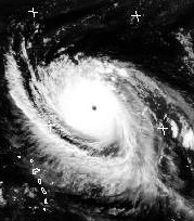
Claudette moved very slowly, first west, then north, then west again, reaching the Texas coast 52 miles south of Galveston in the morning of 15 July 2003. The northward move was unexpected, since the track prediction of 13 July showed a path directly westwards toward Brownsville. Upper winds were generally easterly at 500 mb. The winds had intensified because of the long residence over warm Gulf water, and Claudette was first identified as a hurricane on the weather map for 15 July 12Z (about 6 am CST), with winds of 65 kt. 64 kt promotes a T.S. to a hurricane. The picture is an infrared image from GOES-East, from the Dundee satellite station. The eye is just visible, and its darkness shows it is cooler than the surrounding clouds. The two long spiral rain bands make it look very much like the hurricane symbol. The pressure at 250 mb had been low until Claudette became a hurricane and developed an eye, when the pressure was shown as a low at the 250 mb level. This probably was a result of the increasing altitude of the centre of the storm. After Claudette made land, there was no upper-air indication of her presence at all, showing that when the warm water was withdrawn, the convection subsided. The winds were strongest at low levels, moderating at higher levels, opposite to the usual trend.

The track predictions for Claudette from 12 July are shown at the right. Claudette was predicted to make land around noon on the 15th near Brownsville and remain a tropical storm until the 16th. The track predictions for 16 July are shown at the left, and show the actual path of the storm. Note that the eastern part of the map is a satellite image. Claudette is seen to have continued to move northwestwards, making land near Port O'Connor 52 miles south of Galveston. This map shows the rapid weakening of Claudette over land, which again became a tropical depression between 00Z and 06Z on the 16th. Though the winds were moderated, rain and flooding were still widespread. At 06Z, Claudette was represented as a low of 1000 mb, which had filled to 1004 mb by 12Z. Isobars showing the low pressure at the center of the hurricane are apparently too local to show on a large-scale weather map, and I have not come across the central pressure in Claudette at landfall. Claudette, the first hurricane of the 2003 season, seems to have been a very typical small hurricane.

The closest that hurricanes come to my personal experience is that I have visited Galveston, where there was a disastrous hurricane on 8 September 1900, whose isobars I saw in a old textbook on meteorolgy long ago. They were circular and very tightly packed, again demonstrating the relation between pressure and wind velocity. The minimum pressure was 931 mb, the maximum winds were about 26 km from the centre, and the storm moved at about 6 m/s. The large-scale forces must have been predominately geostrophic, because hurricanes blow clockwise in the southern hemisphere, but cyclostrophic forces predominated at the centre of the vortex. Note that since tornadoes are governed by cyclostrophic forces, they can rotate in either direction around a low pressure core, with the direction usually established by any prevailing vorticity. Hurricanes are driven by the heat released by condensation of water vapour, and depend on a warm ocean surface to give them lots of water vapor. The central eye is a descending column (unlike the centre of a tornado), the whole thing like a toroidal vortex. Each area that breeds hurricanes seems to have a different name; "hurricane" is the Atlantic word, "typhoon" the Pacific. "Cyclone" is used in the Indian Ocean, and "baguio" around the Phillippines. In Australia the term "willy-willy" is sometimes used. Our word "hurricane" comes from the Spanish huracán, a Caribe word. Christopher Columbus first brought the awareness of hurricanes to Europe.

A thin layer of moist air at the surface of the ocean is driven by the pressure difference to converge at the centre of the storm. Before it arrives there, it is caught up in the vortex and rises in the eye wall, releasing its latent heat to drive the upward flow. When it reaches the top, it diverges radially, as the characteristic bands of cloudiness, that curve to the right in response to Coriolis forces, to return to sea level at a distance of 500 to 1000 km. A convergence occurs at about 200 mb that produces cirrus that is sucked into the centre of the vortex, making the relatively clear eye of 10-80 km radius, averaging about 35 km. The energy released in the winds is only a small fraction of the latent heat available in the rising moist air. The sea surface must be heated to about 27°C before evaporation is rapid enough to initiate a hurricane. Hurricanes begin in a tropical low-pressure area where cumulonimbus cluster in a region of high sea surface temperature. Conditions as yet poorly understood cause this area to converge and shrink into a powerful vortex, something that does not happen in mid and high latitudes, because of the lack of the warm sea.

A good qualitative explanation of that curious feature of the hurricane, the eye, would be very welcome, but as I have not found one so far, I shall attempt to construct one. The hurricane is very much like a classic vortex, with linearly increasing wind speed in the eye up to the radius of maximum winds, then wind speed decreasing as 1/r beyond. The flow is cyclostrophic, pressure gradient and centrifugal forces balancing at every point. This model, however, gives no account of what maintains the forced vortex in the centre. In the hurricane, the velocity outside the eye goes more like 1/r^0.6. Friction with the ocean surface retards the flow, causing the velocity to decrease, and so the balance of centrifugal and pressure gradient forces is disturbed, and the velocity turns inward to find regions of higher velocity. This is the spiral inflow of moist, warm air that drives the hurricane. Friction continues to help this air toward the centre, the tangential velocity steadily increasing.

The central pressure determines the maximum pressure gradient, which must increase inwards to balance the increasing centrifugal force. For any central pressure, there is a maximum velocity that can be supported, and when the incoming air attains this velocity it can go no farther, and cannot enter the area of smaller radius, which becomes the eye. It must, however, go somewhere, and the only possibility is up. The air rises, cools and condenses, releasing latent heat and forming the towering eye wall cloud, still spiraling as it climbs. At the top of the storm, a dome of high pressure over the eye presses the air outwards, forming the outgoing spirals of cirrus cloud seen in satellite photographs. The eye is formed like the eye in the water draining through the plug hole in a basin, except that the hurricane is upside-down, the discharge being at the top. Eyes are from 5 km to 60 km radius. A quantitative explanation would relate eye diameter to central pressure, but this seems to be a difficult problem, affected by many factors, including the latent energy release.

Hurricanes occur along the western boundaries of the Atlantic and Pacific oceans, in both northern and southern hemispheres, except for the South Atlantic, which has no hurricanes. Eastern Pacific hurricanes are actually Caribbean hurricanes that have crossed over the narrow land bridge and move northwestwards until they find the cold California Current and die. Hurricanes also occur in the Arabian Sea and the Gulf of Bengal, where there are two hurricane seasons a year, corresponding with the monsoons. Tropical cyclones in the Bay of Bengal are particularly devastating, because of the low coastal plains and the dense population. Australia is assailed by hurricanes from the Indian Ocean, the Coral Sea and the Pacific. Hurricanes generally seem to ride on the anticyclonic flow of the large oceanic highs, "recurving" to accompany them along coasts to the west. However, the paths of hurricanes are highly unpredictable for individual storms. Before modern weather reports were available, hurricanes were anticipated when the weather grew suddenly clear and the normal easterly trades shifted to westerly winds. Satellite images of clouds and temperatures in the high atmosphere have been of great aid in hurricane study. The outflowing cirrus seen in the photographs hides the incoming rain band clouds near the surface.

The next hurricane of the 2003 season after Claudette was Fabian, which began off the southern Cape Verde islands in the last week of August as Tropical Depression Nine. On 1 September it was 460 miles east of Barbuda, and a full Category 4 hurricane with maximum winds of 120 kt or 62 m/s. Its Beaufort number, calculated by the formula, is 18, which is just off the scale. Fabian is shown in the satellite image at the right, a GEOS image from Dundee. The eye is very well shown, and I was able to estimate its diameter as 24 km. The diameter of the circle of maximum winds is probably about twice this. The bright clouds shown are the outflow cirrus clouds at high altitudes; the inflow rain band clouds are close to the surface and darker. Perhaps some are seen to the southeast. The outflow can easily be seen in animated TV satellite photos. Fabian is predicted to begin recurving northward, pass east of the Bahamas, and aim for Massachusetts, with winds decreasing to 110 kt when east of Cape Hatteras. This is a typical strong Atlantic hurricane, while Claudette was a Gulf hurricane.

The diameter of the central cloud disc of the hurricane, scaled from the satellite image, is about 295 mi or 472 km. It moved from 460 mi east of Barbuda on 31 August to 335 mi northeast of Barbuda on 1 September, or 198 miles, so its rate of progress is about 8.2 mph, 3.7 m/s or 13.2 kmph. This means that the storm will require about 1.5 days to pass a given point, and the eye will take 1.8 hr. Fabian is an impressive storm, probably similar in size to the famous one that struck Galveston a little more than a century ago. While Fabian was cruising the north Atlantic, a north Pacific hurricane, Jimena, was at 18°N, 153°W, threatening Hawaii. This storm apparently crossed over from Baja California, where a tropical storm was reported a week ago. I have not yet caught any Pacific hurricane leaping overland from the Caribbean, but it is said that they originate in this way.

Fabian did indeed recurve and begin to move northwards, passing over Bermuda on 5-6 September with winds of 108 kt, about as predicted, as Category 3. The central pressure was 946 mb. This was the strongest hurricane to strike Bermuda since 1953. It passed east of Newfoundland, 680 miles ENE of Cape Race, as a post-tropical cyclone with maximum winds decreasing to 65 kt on the 8th. On the 9th, Fabian had disappeared southwest of Greenland. Fabian was followed about four days later by tropical storm Henri, which began as a tropical depression in the northeast part of the Gulf with winds of 25 kt, passed over Florida, and strengthened as it entered the Atlantic, with winds of 35 kt. By the 9th, it was merely a rainy low.

Meanwhile, the depression that became hurricane Isabel originated near the Cape Verde islands, strengthening as it moved westward. It reached hurricane strength on the 8th, and moved steadlily westward toward the Leeward Islands along the 20° parallel. Meeting cooler water in the wake of Fabian, whose path it followed, the winds were expected to decrease a little, but instead maintained themselves and even increased. On the 8th, Isabel was about 550 km in diameter, with an eye about 20 km in diameter, and maximum winds of 120 kt. The central pressure was reported at 920 mb when the winds had strengthened to 140 kt on the 10th, and Isabel became Category 5. Isabel is shown in the IR satellite photo on the 12th. Because of a strong high to the north, Isabel did not recurve like Fabian, and continued on a northwesterly course. Meanwhile, tropical depression 14 organized itself 220 miles south of the Cape Verdes on the 8th, and moved northwestwards, uninterested in crossing the Atlantic, eventually dissipating. The tropical storm season of 2003 picked up steam in September, and is providing many excellent examples of tropical storms. Most of the activity can be seen from the GEOS-East satellite.

Isabel was an excellent example of a typical strong Atlantic hurricane. Early predictions were for a decreasing intensity and a path that would follow Fabian. When its intensity increased and it moved rapidly westwards these predictions were revised and the new predictions, for a central pressure of 955 mb and 90 kt winds at landfall in the Carolinas, turned out to be substantially correct. On the 18th, Isabel's eye made landfall near Cape Hatteras with 957 mb and 90 kt winds. Isabel's forward progress had slowed abruptly on the 14th, and it began to turn northwestwards on the 15th at 25°N 69°W. On the 17th, it was moving steadily NNW at about 5 kt and 957 mb. Isabel did not strengthen when over the Gulf Stream, but did maintain its wind speed. The weather map showed 5 or 6 closed isobars around its centre. Public interest increased rapidly as the storm approached, and hurricane websites became clogged.

The 250 mb charts never showed any considerable trace of Isabel. Surface winds gave little clue to its progress, so mid-level winds must have been the dominant influence. The encounter with westerly winds as Isabel slowed and turned to the north was notable. Isabel moved almost directly towards a strong surface high with adverse winds. The hurricane models seem to have been very successful, however, especially in the short term.

After landfall, the storm moved almost exactly northward, speeding up and losing intensity. At 02Z on the 19th, Isabel was reclassified as a tropical storm, and at 13Z was at 40.5°N, 79.2°W, 85 km east of Pittsburgh, with central pressure of 986 mb and 45 kt winds, moving NNW at 20 kt. Isabel passed east of Cleveland and moved into Ontario, where it became an extra-tropical cyclone, moved more easterly, and merged with an existing low-pressure area. The storm existed for about 14 days, in which it moved from west Africa to northern Québec. The major effect of the storm was heavy rain over a very wide area, and wind damage in the early part of its path overland.

One thing that should always be kept in mind when dealing with atmospheric phenomena is the predominant influence of the oceans, which is so obvious with hurricanes. Compared to the oceans, the atmosphere is only a small reservoir of matter, energy and gases such as water and carbon dioxide. Even ocean life is important in these matters. The predominant influence is that of the oceans on the atmosphere; the reverse is negligible, though winds affect ocean currents. Ocean currents and water temperatures have more influence on climate than do purely meteorological parameters. Whether the earth is cooling or warming has more to do with the oceans than the atmosphere and its short-term dynamics. This is beginning to be realized, as Reference 2 admits, but meteorology is greatly lacking as a science of climate dynamics. Geologically, we are near the end of an interglacial epoch. Generally, the earth has been warmer than it is now, but there have been persistent cold snaps in the past few million years.

The Beaufort wind scale was devised by Comdr. Francis Beaufort (1774-1857), RN on 13 Jan 1806, when he commanded HMS Woolwich, and revised the following year, to aid in estimating wind speeds from the condition of the sea's surface. Similar procedures had existed for a long time, but Beaufort's was well thought-out and well-documented. He used it privately for a number of years, but it was finally officially recognized in the 1830's when the state of the sky and the Beaufort wind number were ordered to be recorded hourly in the ship's log. Reed's Nautical Companion gives photographs of the sea's surface for each wind force, so that the force can be estimated by simple observation. The table below shows the Force numbers, the corresponding range of wind speeds in knots, and typical land phenomena for estimating wind speed. The whole idea of the Beaufort system is the estimation of wind speeds without instruments. The wind speeds change significantly with altitude, and constantly fluctuate, so precision is worthless. In fact, a single number gives little indication of the state of the wind. The standard height of the anemometer was 30 feet, then 11 metres in the US and Britain (it now seems to be 10 metres). The scale gives a good idea of the range of wind velocities met with in the field, and is useful for the interested observer. The speed of the wind can be estimated from the formula v = 1.87 B^3/2 mph, where B is the Beaufort number.

The Beaufort Wind Scale (Land)

Force	Knots	Description
0	< 1	Calm: smoke rises vertically
1	1-3	Light air: smoke drifts; vanes not moved
2	4-6	Light breeze: felt on face, leaves rustle, vanes moved
3	7-10	Gentle breeze: leaves in constant motion, light flags extended
4	11-16	Moderate breeze: dust, loose paper blow about, small branches moved
5	17-21	Fresh breeze: small trees in leaf sway, water surfaces ruffled
6	22-27	Strong breeze: wires whistle, large branches moved, umbrellas unmanageable
7	28-33	Moderate gale: whole trees move, walking against wind inconvenient
8	34-40	Fresh gale: twigs broken, walking difficult
9	41-47	Strong gale: chimney pots, slates, shingles disrupted
10	48-55	Whole gale: trees uprooted, some structural damage. Seldom on land.
11	56-63	Storm: damage widespread. Very rare on land.
12-17	64-118	Hurricane: flooding, devastation.

Names that are used to describe wind strengths are shown in the table. There is a poverty of words to describe winds of different strengths, reliance being placed on adjectives. It is better to give the Force number.

The wind speed was of critical importance to sailing ships, because it controlled the amount of canvas they could safely carry. A Force 1 wind was just sufficient for steerage way (for the ship to respond to the rudder). A ship could carry all sail in Force 2-4 winds. In Force 5, the royals had to be taken down. Force 6 required a single reef, Force 7 a double reef, Force 8 a triple reef, and Force 9 a close-reef. In a Force 10 wind, a ship could carry only a close-reefed maintop and a reefed foresail, and in Force 11 only storm staysails. No canvas at all was to be carried in Force 12 and stronger winds. Reef points were short ropes attached to the sails at intervals. A single reef used the first set, a double reef the second set, and so on. When too much sail was set, a ship would labour, or roll and pitch, causing great strain in the masts, rigging and hull, opening seams or even dismasting the ship. A staysail was a triangular fore-and-aft sail set on a stay (support for a mast). Navigation using the winds as propulsive power is an ancient and remarkable thing, and was brought to great perfection.

The wind exerts a force on bodies moving relatively to it, and we may want to estimate the force. To find the force on a plane surface normal to the wind, we can use the impulse-momentum principle mΔv = FΔt. The amount of momentum transferred to the surface in a time interval dt is (ρV)(Vdt) per unit area, which must be equal to the pressure P times dt, or P = ρV². This actually overestimates the pressure, so it is a useful formula for engineering purposes. The density of air at STP is ρ = 1.293 x 10^-3 g/cc. For a wind of 10 m/s (33 ft/s) P = 1293 dyne/cm² or 2.7 lb/ft². The pressure is easily calculated for any wind velocity you wish. If the air strikes the surface at an angle θ with the normal, the pressure is multiplied by cos²θ.

The force on a body of projected area A is expressed as F = CAV²/2, where C is the coefficient of drag. If, as is the usual case, the flow is turbulent (Reynolds number Re = 2rV/ν > 1, where 2r is the diameter of a spherical body), the body creates a turbulent wake behind it, and the force is due to the difference in pressures on front and back. This is called form drag. C is a function of the Reynolds number, and is different for bodies of different shapes. For laminar flow, at small Reynolds numbers, C = 24/Re. For a sphere at moderate Reynolds numbers, C = 0.5, approximately, and for a disc, C = 1.0. A streamlined body makes only a thin turbulent wake, and C can be as low as 0.04. These figures are good enough for estimates, but for accurate values the aerodynamical literature should be consulted.

When a nonspherical body falls freely, it orients itself for maximum C. This is easily tested by dropping light objects, such as leaves. A disc, therefore, falls so that its plane is horizontal. For such bodies, C can be taken as 1 for the purpose of estimates. This applies particularly to ice crystals in the form of plates, which is very common. The crystals falling from cirrus clouds will all have the same orientation, facilitating the creation of halos, which are the cooperative effect of many crystals (as the rainbow is of many drops). An ice crystal should fall more slowly than a droplet of the same weight, jointly due to the increased area and the orientation.

The terminal velocity of falling spheres is of some interest in meteorology, so it will be discussed here. At the terminal velocity, the drag is equal to the weight of the body, and can be found in this way. The drag is F = C(ρV²/2)A, while the weight is (ρ' - ρ)gv, where v is the volume of the body and g is the acceleration of gravity. ρ' is the density of the body, which for water is 1. This gives V² = 2F/ρCA = (16/3)(ρ' - ρ)gr/ρ, where we have used C = 0.5, v = 4πr³/3 and A = πr². The terminal velocity is V = 6.36r^1/2 m/s, where r is in mm.

The Reynolds number is Re = 133r(mm)V(m/s). When this is less than about 10, the drag coefficient rises when the flow changes from turbulent to laminar, and is equal to 24/Re. With this value of C, we find a terminal velocity of V = 112.3r² m/s, again with r in mm. The two formulas give the same terminal velocity when r = 0.147 mm, when V = 2.44 m/s and Re = 47.7. This is a reasonable choice for a dividing line between turbulent flow for larger spheres, and turbulent flow for smaller spheres. The terminal velocity does not vary smoothly through this region; when laminar flow occurs, the drag increases abruptly and the terminal velocity abruptly decreases. In turbulent flow, the terminal velocity does not vary rapidly with r, but for laminar flow it does.

Raindrops have diameters between 0.5 and 5.0 mm. We see that the flow is turbulent, and these drops fall rather rapidly, from 4.5 m/s to 14.2 m/s. A more accurate investigation would put the upper velocity closer to 8 m/s, allowing for the flattening of the larger drops and the consequent increased drag. Drops of this size get out of the air rapidly. Fogs and clouds have droplets with diameters between .004 and .030 mm (4μm to 30 μm). These are definitely in the laminar flow region, and fall at rates of 0.18 cm/s to 10 cm/s. In an hour, the fastest of these would fall only 360 m, and the slowest only 6.5 m. Clouds, and fogs, are actually falling at these rates, but slight turbulence keeps them suspended.

Intermediate between rain and fog is drizzle. Drops with diameters from 0.1 to 0.5 mm may be in either the laminar or turbulent range, more probably the turbulent, so they will fall with velocities of around 1 m/s, and will make one quite wet, while being too small to be easily seen.

Rain and drizzle have drops much larger than the wavelength of visible light, so they will not show evident diffraction effects. They will, however, exhibit the rainbow and other reflection-refraction phenomena, as will ice crystals. The particles in fogs and clouds are much smaller, so they may show diffraction effects, as well as small-angle scattering in any case. Fog and cloud particles are still many wavelengths in diameter, so the scattering will be independent of wavelength. The color of light has no effect on visibility in fog; no color "penetrates" fog better than any other, but some colors may give improved contrast. The smallest particles, only a few wavelengths in diameter, produce colored halos and other diffraction phenomena. This is especially seen near the edges of clouds, where the particle size may be expected to be small. However, the cloud must be thin, and the particles of roughly equal size, for a good effect.

When vapor, water and ice are simultaneously present in a cirrocumulus cloud of supercooled water droplets, the droplets evaporate in favor of ice crystals because of the difference in vapor pressure, and so the ice crystals can grow while the droplets could not. The larger ice crystals then fall rapidly out of the bottom of the cloud, making the typical cirrus fibers. It does not take long for the cirrocumulus to dissipate into falling ice crystals, which then melt and evaporate in the dry, warmer air below.

If these ice crystals should fall into a warm lower cloud containing much moisture, they melt and then grow as they fall, sweeping up droplets in their path, and falling as rain. This is known as the Bergeron process, after Tor Bergeron, who conceived it in 1928, and published it in 1934. The Bergeron process competes with growth and coalescence of droplets in clouds above 0°C, which can create drizzle in nimbostratus, and rain in tropical convective storms. In middle and high latitudes, the Bergeron process is responsible for nearly all rain, but the role of competing processes is now recognized.

Raindrops, and even hailstones, can be supported by updrafts of a velocity greater than the terminal velocity, which is not very difficult for the smaller drops. This plays a role in the complex phenomena of the cumulonimbus. Electrical charge is separated when water droplets are formed, and this causes lightning and a thunderclap. Then the large droplets fall to earth from the cloud base at 1 km in 2 minutes, followed a minute later by the smaller drops. This familiar succession can be noted in many thunderstorms.

1. A. E. M. Geddes, Wind Structure, in C. V. Drysdale, et. al., The Mechanical Properties of Fluids (London: Blackie and Son, 1925).
2. Dick File, Weather Watch (London: Fourth Estate, 1990), a comprehensive survey of meteorology, specializing in British weather, which naturally has lots about winds and pressures, and much else. There is absolutely no mathematics to frighten the children, but it is quite accurate and intelligent. Meteorology is an excellent school subject, which he underscores. Newer aspects, such as computer modelling and satellite observations, are included.
3. E. W. Hewson and R. W. Longley, Meteorology Theoretical and Applied (New York: John Wiley & Sons, 1944).
4. R. H. Simpson and H. Riehl, The Hurricane and its Impact (Baton Rouge, LA: Louisiana State University Press, 1981).
5. All my weather information comes from the Canadian Weather Office, and satellite images are from the Dundee Satellite Station, whose generosity is gratefully acknowledged.
6. The National Weather Service Hurricane Center is at NHC. This is better than most NWS web information. An extensive list of worldwide hurricane names is included.

Composed by J. B. Calvert
Created 30 July 2000
Last revised 3 April 2004