Processing GPR Data

Each two-dimensional reflection profile will show you much about what is below the ground, but if you have more than a few in a grid (which is almost always the case!), correlation of reflections from profile to profile, and throughout a large area, can be laborious.   For this reason there are a number of techniques that have been used to help with processing and ultimate interpretation.

Reflection Profiles

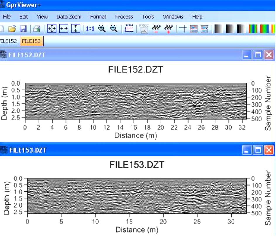
Jeff Lucius and I (mostly him!) are working during Summer and Fall, 2010 on a new GPR Viewer program that will allow you to produce interactive reflection profiles.  The old program, written in Java is great, and most of us still use it.  But it took up much memory, was not compatible with some new Windows versions, or OS-2.  So the plan is to reformulate the whole program.  Here is an example of what that program does at a Roman site in Israel:

 If you need a copy of this old program, e-mail me, and we will work something out.

Amplitude slice-mapping

This is a method that is now commonly being used to process large data bases.  In general the computer is used to analyze all the amplitudes of reflections in all profiles within a grid, and then make maps of the relative spatial distribution of these amplitudes, within discrete slices in the ground.  This is done by telling the computer the search radius you want to look for amplitudes both along profiles, and between profiles (in meters or sub-meter distances), and also what thickness you want to search for those amplitudes (usually in nanosecond thicknesses).  When this is done a number of slices, superimposed on top of each other will show the relative reflections of what lies at specific depths in the ground.  The slicing data is computed with my own software that you can download from this site by clicking here, and the maps are made with Surfer, a wonderful software program from Golden Software.   Dean Goodman also sells a software package for slicing, that will make maps and many other images. Here is an example of some slices from Japan that Dean Goodman made back in about 1995.

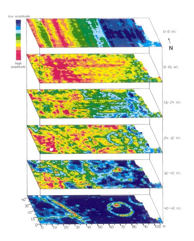In this picture you can see plow marks on the near-surface slice, but as you get deeper in the ground, the circular outline of a burial moat around a deeply buried burial chamber.

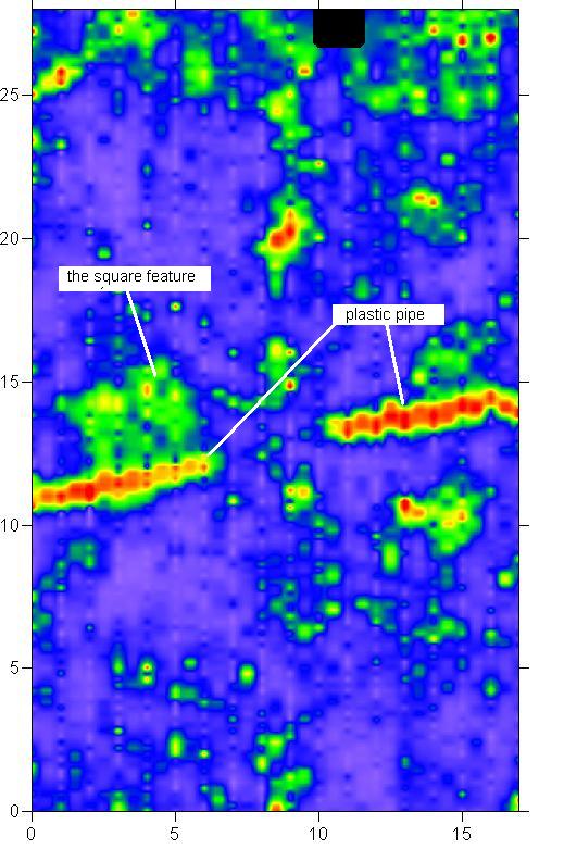
When looking for a buried fiber-optic conduit, this same method can be used, as these two slices show, with the upper slice being near the surface, and the lower one about 3 feet buried in the ground.

Often we take these slices and decide which is the depth that is of interest to us, and then superimpose it on what we know from the surface.  At this historic site on Whidbey Island, Washington, the reflections are placed on a map an old farmhouse, and the nature of the reflections in the ground can be seen spatially. 

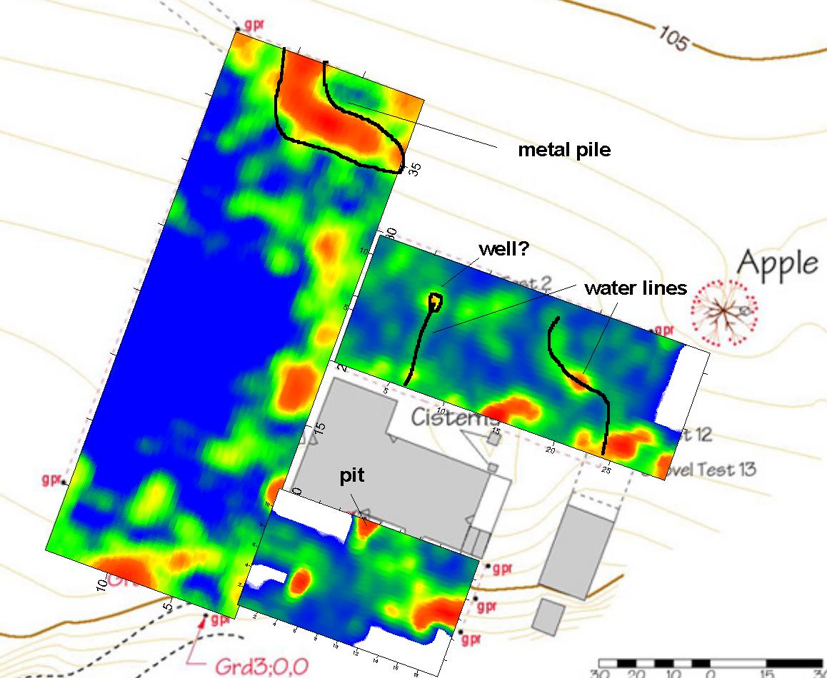
All anomalies in this map are probably buried metal and pipes, but we think some could be prehistoric baking ovens and other features of this sort.

This is another good historic example, showing where buried foundation walls, made of stone and concrete, are at the Angel Island California Administration Building, which was destroyed by fire and buried many decades ago.

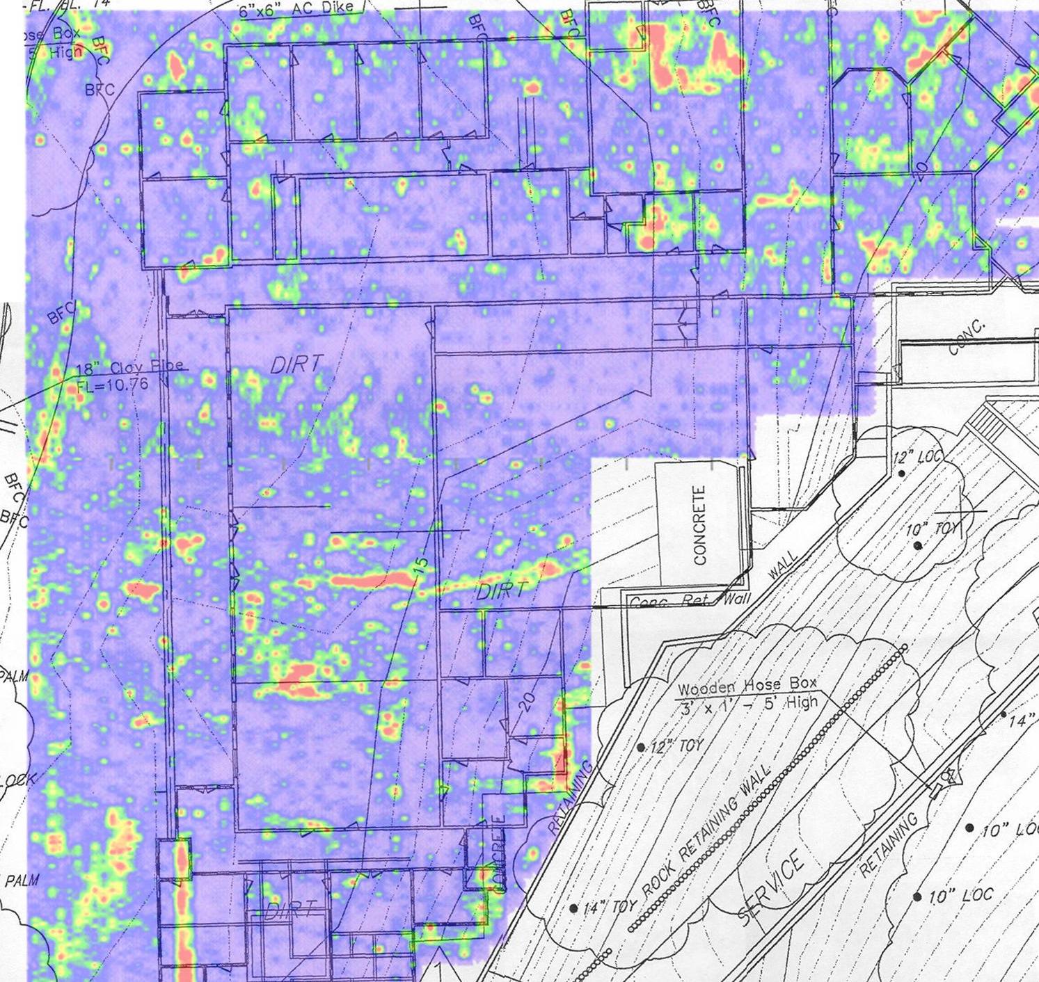
In this picture the slice from about 80-100 cm in the ground is placed on an old blueprint of the building.  It is then easy to see which of the rooms and foundations are still present, and where the piles of rubble from the building construction are located.

Sometimes it is helpful to compare GPR maps to maps prepared from other geophysical tools.  At the San Marcos Pueblo south of Santa Fe a magnetic gradiometer map was compared to one GPR slice.  The GPR map is on the bottom and the magnetic map is on the top. 

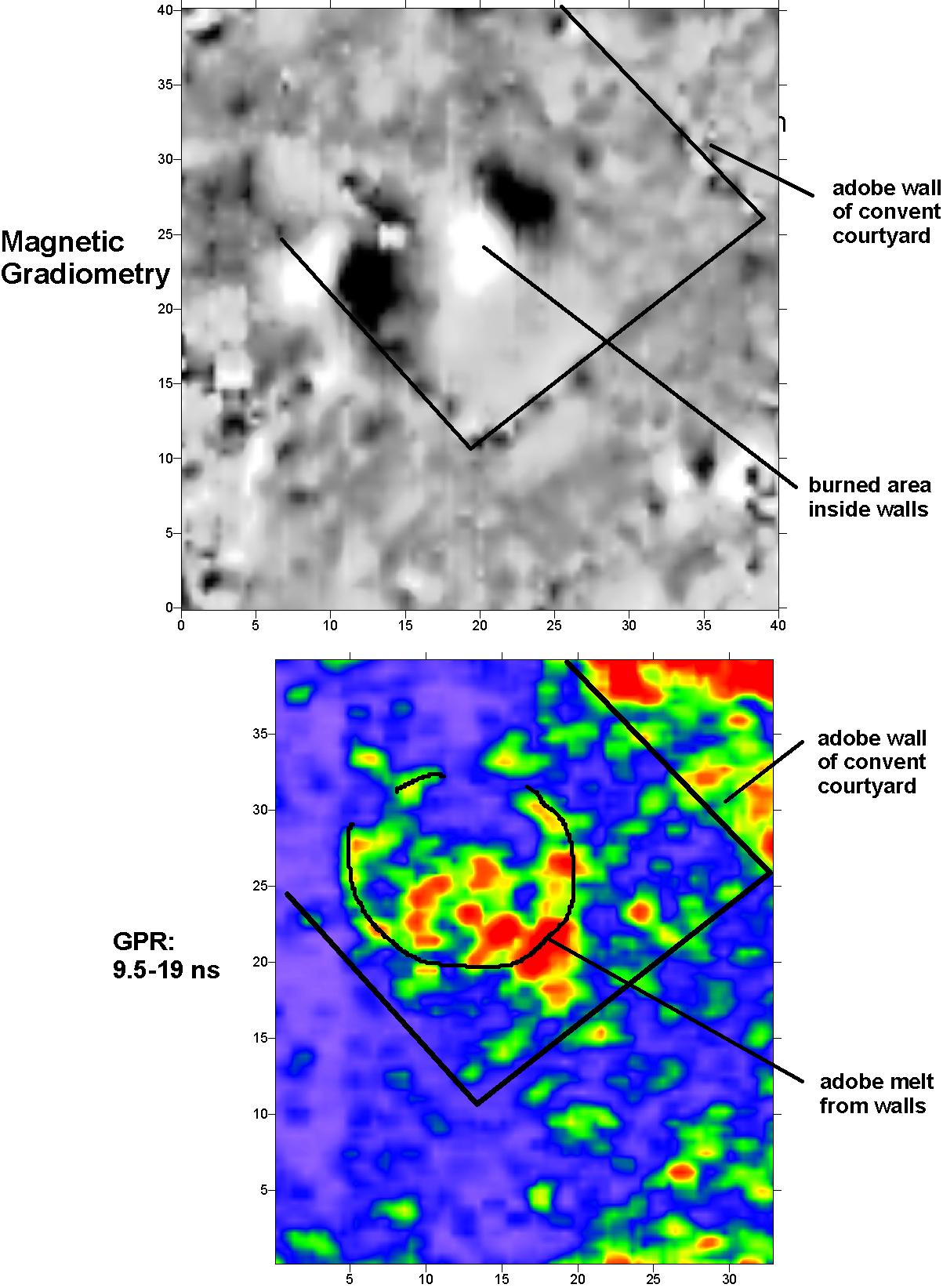
The GPR map appears to show a circular area filled with high amplitude material, which the magnetic map is showing it is burned.  We hypothesized it was a circular "kiva" or pit house that might have been burned in the past.  We excavated it to see what this was, and found it was a depression created by the "melting" of adobe walls that was filled with cow manure and buried!  Not at all what we expected, but interesting that these two tools, working in conjunction, could determine this.

When many thin slices are produced, then can be processed in three-dimensional rendering programs that will produce images of the highest (or lowest if you prefer) amplitudes in a grid.  Here is an image of buried construction material...not too exciting, but it was close to my campus. 

Buried in a parking lot is the foundation of a 19th Century building, and we go there to practice different tools.  Individual rocks and buried metal objects can be seen in this image.  It was produced by a program called Slicer-Dicer, sold by Pixotec Inc.