A Magnetometer
Measuring magnetic flux from 15 to 2000 gauss
Introduction
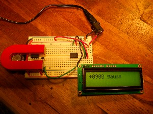 It is easy to measure moderate magnetic fields using a Hall sensor, such as the Allegro A1302 linear Hall sensor, available from Jameco. A PIC12F675 can digitize the output of the sensor and display it on a serial LCD display, such as the Newhaven NHD-0216K3Z-FL-GBW 2 line x 16 digit display. This system is shown breadboarded in the figure at the right, measuring the field between the poles of a horseshoe magnet.
This instrument is not suitable for measuring weak fields, such as the geomagnetic field. Compass modules contain magnetometers of appropriate sensitivity, however.
The Hall Effect Sensor
Although we will not need to understand the details of the Hall effect for this project, it is interesting to review how it arises. It was discovered by Edwin H. Hall in 1879 in the course of research for his PhD thesis at Johns Hopkins under Prof. Rowland. It is the creation of an electric field perpendicular to the directions of the magnetic field and an electric current when the current flows in the presence of a magnetic field. In the simplest configuration, the current is assumed to flow in the x-direction while the magnetic field is in the z-direction. The Hall field is then in the y-direction, where xyz form a right-handed basis.
The force on a charge q in electric and magnetic fields is given by the Lorentz equation, F = q[E + v x B/c] in Gaussian units. In equilibrium, the force will vanish, so that E = -v x B/c. IN our simple geometry, this is Ey = vxBz/c, independently of the sign of the charge. However, the velocity will be in opposite directions for opposite signs of the charge carriers, and so will be the Hall voltage. Now, jx = Nqvx, where N is the density of charge carriers and q is the signed charge. Therefore, Ey = (1/Nqc)Bzjx. The coefficient (1/Nqc)By is the Hall resistivity, and 1/Nqc is the Hall constant, which is -1/Nec for electrons, a negative number. If we measure the Hall voltage, we can infer the magnitude of the magnetic field B if we know the Hall constant. This is how the Hall sensor is used in this project. In solid state investigations, we can obtain information about charge carrier signs and concentrations from the Hall effect.
 Metals usually have small negative Hall constants agreeing well with otherwise known electron concentrations. However, there are surprsing cases of positive Hall coefficients in Zn, Cd and Be which are explained by hole conduction. Semiconductors have large Hall coefficients because of the small carrier concentrations, and they can be of either sign depending on whether the majority carriers are electrons or holes.
The sensor contains the Hall element, a current source and an amplifier. The output voltage is 50% of the supply voltage, 2.5 V with a 5 V supply, with no magnetic field. The output voltage varies linearly with flux density above and below this voltage depending on the direction of the field, with a sensitivity of 1.0 - 1.6 V/gauss, the typical sensitivity being 1.3 V/gauss. The supply current is about 10 mA. The pinout is shown at the left. The sensor can easily be tested with a DMM.
The LCD Display
The Newhaven serial LCD display offers the input options of an asynchronous link or, if jumpers are soldered in the proper places, an SPI or I2C link. The asynchronous link is so convenient that there is no reason not to use it, and it requires only one wire. The default speed is 9600 bps, which is also quite satisfactory. The display uses a PIC16F690 to handle the serial interface, communicating with the parallel display controller for the LCD. The serial displays are a little more expensive than the 8-bit or 4-bit parallel interfaces, but are very convenient and economical of MCU pins. We have already shown how to use the 12F675 8-pin MCU to handle asynchronous communication. Note that pin 1 on the connections is identified by a square solder pad. We use only the 3-pin connection; from the end, the connections are TX, Gnd and VDD.
Commands to the display are preceded by an 0xFE prefix byte, followed by the command byte, which in some cases is followed by one or more data bytes. All other bytes will be displayed at the current cursor location according to the font table, which includes Roman letters, Japanese katakana, and a few Greek letters. Cursor address 0x00 begins the first line, and 0x40 begins the second line, on a 2-line display. Characters will be displayed in the first 16 or 20 positions, but can be written beyond this. The display window can be moved to the right or left. Underline or flashing cursors can be displayed or hidden. The cursor can be homed, moved to any address, or moved right or left by one space, to control where characters will be displayed.
The default display contrast is 40, which shows the character arrays dark against the background. I found it more suitable to reduce the contrast to 20 with the command sequence FE 52 14. The backlight brightness was satisfactory.
Eight user-defined characters can be displayed by sending bytes 00 to 07. To define the characters, 9 bytes are sent after the command FE 54. The first is the character number, and the next 8 are the bit-map of the 5x8 character, as shown in the data sheet. I found that defining a character interfered with the display, but this can be overcome by defining the characters first, then homing the cursor for further use. Clearing the screen had the same effect.
The display is very easy to use. Simply clear the display and send the desired characters. It is convenient to have a table in the program converting hex digits 0-F to the corresponding characters, for use when displaying numbers.
Programming the Processor
Because of the asynchronous communication, it is necessary to use the factory oscillator calibration to load OSCCON. Only the asynchronous transmitting routine is required here.
The output of the Hall sensor can be connected to AN0, pin 7. The AD converter is configured to use AN0 for input, VDD for reference, and left-justified . For simplicity, I used just the 8-bit result from ADRESH, but the full 10 bits can be used for better precision. At power-on, it is assumed that no magnetic field is applied, so the first conversion is saved as the zero-field reference value. The program then enters a loop in which the output of the sensor is read and then displayed in gauss. The reading is subtracted from the reference value. If the result is negative, the fact is noted, and the difference converted to a positive value. Assuming a sensitivity of 1.3 mV/gauss, The value of each bit in gauss is known. Each bit is then tested, and the value of each 1-bit is then added. The sum will be the field in gauss, which can then be displayed. The routines for doing this bit testing and 4-digit decimal addition that we have already used, as in the humidity meter, apply here as well.
References
Data sheets for the Hall sensor and the LCD display can be obtained from the Jameco website.
The Hall effect is described in C. Kittel, Introduction to Solid State Physics, 2nd ed. (New York: John Wiley & Sons, 1956), pp. 296-301.
Return to Electronics Index
Composed by J. B. Calvert
Created 21 October 2010
Last revised