• A Geophysical Survey Systems Inc. (GSSI) Subsurface Interface Radar (SIR) 2000 system was used to generate and collect the radar data.
  Figure 14
  
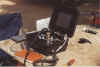
• A 400 MHz antenna was used to transmit energy into the ground, receive the reflected pulses, and transmit it to the base station.

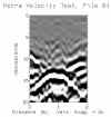
• Velocity tests are necessary for each site to obtain radar pulse travel times.
  Velocity can then be used to convert travel time to true depth of reflections in the ground.
• A series of velocity tests were preformed just northwest of GPR Grid 1.

• To perform these tests the 400 MHz antenna was used to collect a short transect over a metal bar that had been inserted at measured depths in the ground.
  Figure 15
  
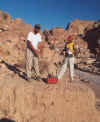
• Metal is a perfect radar reflector and is visible on profiles as a distinct hyperbola.
  Figure 16
  
• The initial velocity tests later proved to be inaccurate because the area tested had been exposed in trenches for more than 3 years and the sediment had dried out significantly.  The lack of water made the radar velocities at this location too fast.
• When those inaccurate velocities were applied to the GPR data, the reflections were calculated to be deeper in the ground than they truly were.

• GPR reflection profiles in Grid 1 were collected with a 50-cm line spacing.  A total of 121 transects were collected in an "L" shaped grid.
  Figure 10
  

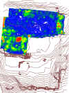
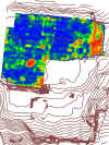
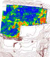
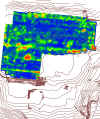
• Amplitude slice-maps were generated on a computer to view all significant reflections in the grid.
• These maps are produced by comparing the reflected wave amplitudes in all the transects within the grids in 25-cm slices.  
  • The highest amplitudes are colored red
  • Areas with little or no amplitude are blue
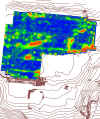
• Six individual slices, each 25 cm thick, were produced.  They are shown below, overlaid by the topography of the "Lower Market" area.  Figure 17 is from 0-25 cm depth in the ground and Figure 18 is from 25-50 cm, while each subsequent slice is an additional 25 cm deep.
  • A number of linear walls, buildings and other features are visible at each depth

Figure 18

• An animation of 45 individual slices starting with the ground surface and going to 2.5 meters total depth was created for Grid 1.  Each slice is about 5-6 cm thick and when viewed sequentially the video shows the spatial distribution of features in map view, and with depth.  You can play the video by clicking on the thumbnail image:
  Figure 23
  
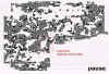
• In Figure 18 shows rectangular structure in the northern portion of the grid.  This building was chosen for more detailed study in Grid 2.

• Grid 2 was collected over the northern structure with 25-cm line spacing and a 20-ns time window for greater resolution.
  Figure 10
  

• Grid 2 data were processed in the same way as those in Grid 1 to produce a video from the ground surface to 2.5 meters depth.  You may click on the thumbnail image below to see this video:
  Figure 24
  
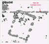
• A distinct rectangular structure was imaged, with possible standing columns on the east and west walls and a more solid northern wall.
• In two-dimensional reflection profiles distinct stratigraphic layers adjacent to the walls were visible, which were hypothesized to be buried garden soils.
  Figure 25
  

• Slice maps, videos and profiles were used to determine placement of subsurface tests in order to confirm features visible in Grids 1 and 2.
  Figure 26
  
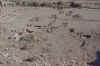
• Test trenches were placed on the northwest corner of the structure in Grid 2 (Trench 8) and the southeast corner (Trench 6).
• Figure 27